omdec.com
http://www.omdec.com/moxie/About/cases/optimizing-a-mine-haul-tr.shtmlOptimizing a Mine Haul Truck Wheel Motors’ Condition Monitoring Program: Use of ProportionalHazards Modeling
This work was completed at Cardinal River Coals in Canada to improve the existing oil analysis condition-monitoring program being undertaken for wheel motors. Key variables were then incorporated into a decision model that provided an unambiguous and optimal recommendation on whether to continue operating a wheel motor or to remove it for overhaul in the basis of data obtained from an oil sample. By optimizing the times of repair as a function both of age and condition data a 20-30% potential savings in overhaul costs over existing practices was identified...
This work was completed at Cardinal River Coals in Canada to improve the existing oil analysis condition-monitoring program being undertaken for wheel motors. Key variables were then incorporated into a decision model that provided an unambiguous and optimal recommendation on whether to continue operating a wheel motor or to remove it for overhaul in the basis of data obtained from an oil sample. By optimizing the times of repair as a function both of age and condition data a 20-30% potential savings in overhaul costs over existing practices was identified...
A.K.S. Jardine*, D. Banjevic*, M. Wiseman § , S. Buck†, T. Joseph*,
*Condition-Based Maintenance Laboratory, Department of Mechanical and Industrial Engineering, University of Toronto
§PricewaterhouseCoopers, Toronto
†Cardinal River Coals Ltd., Alberta
The paper discusses work completed at Cardinal River Coals in Canada to improve the existing oil analysis condition-monitoring program being undertaken for wheel motors.
Oil analysis results from a fleet of 55 haul truck wheel motors were analyzed along with their respective failures and repairs over a nine-year period. Detailed data cleaning procedures were applied to prepare data for modeling. In addition, definitions of failure and suspension were clarified depending on equipment condition at replacement. Using the proportional-hazards model (PHM) approach, the key condition variables relating to failures were found from among the 19 elements monitored, plus sediment and viscosity. Those key variables were then incorporated into a decision model that provided an unambiguous and optimal recommendation on whether to continue operating a wheel motor or to remove it for overhaul on the basis of data obtained from an oil sample.
Wheel motor failure implied extensive planetary gear or sun gear damage necessitating the replacement of one or more major internal components in a general overhaul. The decision model, when triggered by incoming data, provided both a recommendation based on an optimal decision policy as well as an estimate of the unit's remaining useful life (RUL). By optimizing the times of repair as a function both of age and condition data a 20-30% potential savings in overhaul costs over existing practice was identified.
Keywords: Wheel motors, Condition monitoring, Oil analysis, Proportional-hazards modeling, Optimizing condition-based maintenance decisions, EXAKT software
Current practice for monitoring the health of items is through examining trends in readings obtained from various forms of condition monitoring. Interpretation of these readings is undertaken by an inspector reviewing current and past readings, or through using commercially available trending software. Such an approach does not guarantee that the full information-value contained in the readings is captured. The paper uses a statistical procedure called proportional-hazards modeling to identify the key measurements that should be used to assess the true state of health of the equipment. Economic decision rules are then established. The procedure is described through a case study that reports on the optimization of condition-based maintenance decisions for haul truck wheel motors that are monitored through oil analysis. Application of the procedure demonstrated a 20-30% potential savings in overhaul costs compared to current practice.
This paper underlines the importance of data cleaning and applying a consistent definition of failure based on both the observed equipment condition at repair time and the inability of the equipment to perform its functions. (for additional discussion see Campbell and Jardine 2001).
Cardinal River Coals Ltd. is a 50/50 joint venture between Luscar Ltd. and Consol of Canada, Inc. The mine is located approximately 50 km south of Hinton, Alberta on the eastern slopes of the Rocky Mountains. The coal produced from the mine is low sulfur, high quality coking coal used for steel making. Cardinal River Coals Ltd. opened in 1970 as a multiple open pit mine using the truck and shovel mining method. Current annual production at the mine calls for the removal of 21 million cubic metres of rock and 2.8 million tonnes of coal. The mine has won multiple awards for the land reclamation and creating wildlife habitat.
There are 26 haul trucks at the mine site, each having two wheel motors. With 3 spare wheel motors the fleet numbers 55.The existing policy, based on experience, is to rebuild the units after about 20,000 hours of operation. Oil analysis is carried out monthly whereby the amount of sediment (weight of filter patch filtrate) and parts per million (ppm) of five out of the nineteen elements are noted: iron, silicon, chrome, nickel, and titanium. The decision to remove the unit for rebuild is based on manual perusal of the values of these elements in combination with the unit's age.
Wheel motor failures relating to the electrical drive elements and braking system were not included in this study since their condition is not reflected by oil analysis data. Seal replacements were carried out frequently as a result of high contamination and coincided with oil change outs. The oil change out event (OC) is considered as a “minor” repair. The analysis shows that a high amount of sediment persisting in spite of these corrective measures, is associated with a high risk of failure.
Statistical analysis of the CRC wheel-motor data showed a high correlation between iron and silicon. That fact would support the view that there are a high number of failures which are contaminant induced. Hence one may conclude that there is an event or set of conditions that initiate a process of deterioration in the wheel motor. It is assumed that by overhauling the unit before the damage becomes more extensive one would benefit from savings through failure avoidance.
Within the mine’s computer maintenance management system (CMMS) there were histories of wheel motor lifetimes, including details of removals due to failure or preventive maintenance as a result of interpretation of the signals obtained from oil analysis. Costs associated with the failure and preventive removals were also available.
Additionally, there was a database containing a vast history of condition monitoring test results – some 50,000 records.
It may seem that it would be an easy matter to peruse and study these two data sources and learn which patterns of data have been associated with past failure, thus identifying the data combinations that might be employed as condition indicators of future failures. Unfortunately identification of the key condition indicators from amongst all the data collected is seldom obvious to the analyst. The complexity, volume, and time lags within the data render them elusive if not impossible to discern without the proper tools.
In this paper we show a tool that uses a statistical modeling technique known as proportional-hazards modeling to bridge these two invaluable data sources. It is the central function in a program called EXAKT developed precisely for this purpose by the condition based maintenance (CBM) laboratory at the University of Toronto (see Jardine et al, 1997).
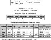
The Weibull-PHM (Equation 1) relates an item’s reliability to its working age and to significant measured variables known as condition monitoring (CM) data.
In Equation 1 h(t) is the (instantaneous) conditional probability of failure at time t, also known as the hazard function, given the values of Z1(t), Z2(t), … Zm(t). Each Zi(t) in represents a monitored condition data item at the time of inspection. These measurements may include the parts per million of iron or the vibration amplitude at the second harmonic of shaft rotation, or any variable that reflects the accumulated stress or damage with respect to some mode of failure. These condition data are sometimes called covariates. The g’s are the covariate parameters weighting the degree of influence each covariate has on the hazard function. The model consists of two parts, the first part is a baseline hazard function (Weibull) that takes into account the age of the equipment at time of inspection, . The second part, , takes into account the key variables and their associated weights.
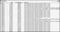
The first step in every proportional hazard model (PHM) building exercise is a thorough examination of the data. The data-cleaning phase of PHM is considered the most important one of the entire modeling process. If we are to accomplish our objective of accurate and automated CBM data interpretation, the data upon which we intend to build the model must be as free of error as is possible. Much of this paper, therefore, focuses on the data investigative or cleansing phase of model building.Fortunately software provides us with ample tools with which to “cleanse” the data. In Figure 1 we show a feature of the EXAKT software (2) that discovers many logical data inconsistencies emanating from the CMMS, thereby helping the analyst to make the corrections that will improve the ultimate model’s precision.
Figure 1 Data checking tool
Data required for PHM analysis consists of "histories" or life-cycles. Each valid history for a wheel motor must have a Beginning event (B), an Ending event (EF for failure, or ES for suspension (such as a preventive removal)) and Inspection events. A discussion of how suspensions and failures were determined is given later in this paper. A history could also have events that are known to affect covariates, such as oil change (OC) events.
The output of the data - checking tool (illustrated in Figure 1) points out probable errors based on a systematic evaluation of working ages and corresponding calendar dates as reported in the CMMS. The software deduces, from the dates and working ages, which inspection and event sets of data comprise individual histories. When it finds a history without an ending reported, it asks whether the ending event should be designated as a suspension (ES), a failure (EF), or whether the the life-cycle has not yet ended. In this latter case, the software assigns it temporary suspension event (denoted by *ES in the software) Temporary suspension means that the item is still operating at the time of the data analysis. Eventually that item, in the future, will end its life either by an ES or EF event.
The software also calls the analyst’s attention toanomalies that may indicate data problems or errors. These will include two inspections on the same date (date and time) or working ages and calendar dates that are out of synchronization. For example an inspection at a later date may have a lower working age than an earlier inspection. This is obviously an error in data transcription, which, if allowed to persist in the data would compromise the model’s accuracy.
Most errors can be easily be corrected, usually simply by inserting missing Beginning and Ending events for each history.
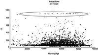
Investigating with the commercial laboratory it was found that for a period of time the photo-multiplier tube on the spectrometer was saturating at exactly 900 PPM. In other words all values of silicon above 900 were truncated to 900 PPM. A similar situation occurred for iron above 2500 PPM. If not detected, this could play havoc with the PHM.
It was possible to compensate for the laboratory errors in preparing the data used to build the model. For example, the truncated values of ‘Si’ they were replaced with 1.2 x Fe. The factor of 1.2 was determined from the initial slope of the cross graph (a correlation graph) of Fe-Si and values obtained after the saturation defect was corrected. The truncated Fe values were not corrected since there were too few of them to influence the model.
The correction applied to the Si values is illustrated in Figure 3.
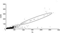
Cross graphs of pairs of covariates are invaluable in finding correlations that are of great help in developing and evaluating the eventual model.
Figure 4 shows the correlation between iron (Fe) and nickel (Ni). Correlations between other covariates were also tested. For example, Fe vs. Ti, Fe vs. Si and Ni vs. Ti graphs all exhibited similar correlation.Determining correlation between covariates is useful both to provide insight into the data and to understand the models generated by the software. For example, if ‘Fe’ and “Ni” are highly correlated the modeling process could indicate that there is no point in including nickel in the model since it has been determined to provide no additional information regarding the probability of failure. These correlation could be the result of wear of a component whose metallic alloy contains both iron and nickel.
Figure 4 Correlating iron and nickel
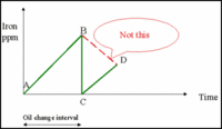
When building the PHM it is necessary that account be taken of any minor maintenance work, such as changing the oil in the wheel motor. For example, Figure 5 illustrates that the actual transition path of oil measurements was from A to B to C to D. If we did not account for the oil change, then the modeling process would assume that the transition was A to B to D. This would be misleading and would tend to overestimate the risk of failure.
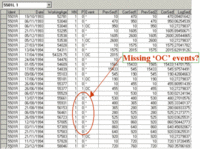
In the EXAKT data preparation phase, the model is told what covariate values should be associated with those minor corrective events, such as an oil change (OC). Such events could include calibrations or cleaning that would tend to reset certain measurements but not materially zero-time the asset. Figure 6 shows ‘missing’ or ‘irregular’ oil changes and obvious gaps. Calculations indicate oil ages of 7000-8000 hours. Such extended oil usage is unlikely given the use of mineral oils in this application. Obviously oil change events occurred but were unreported in the CMMS. The site did change to synthetics recently (1997) in order to eliminate the need for regular oil changes. However most of the data covers the period prior to 1997. It was thought that this information needed to be recovered from the commercial laboratory’s files. Unfortunately these files, too, were incomplete and inconsistent with the dates and working ages in the work order database.
Figure 6 Missing oil change events
Happily, it was determined that these 'missing' oil changes did not significantly affect the model since they were relatively few in number (with respect to all of the known oil changes). That is, there were a sufficient number of known oil changes in the database for the model to account for their effect on the measured data.
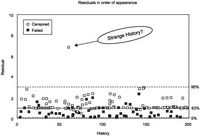
After all the obvious data errors were eliminated or corrected, the proportional hazard model could be generated by the EXAKT software. As illustrated in Equation 1, the hazard function is the short term probability of failure of an unfailed unit at a given point in time. It is a function of both working age and the “significant” condition data. An iterative procedure in the EXAKT software removes the insignificant covariates and weights the significance of those remaining covariates found to influence the hazard. A number of candidate models are then tested to see how well they represent the actual data. One of the test methods used by the software is known as residual graphical analysis illustrated in Figure 1.
Each point on the residual graph of Figure 7 represents a history (the time from wheel motor installation to its removal for whatever reason). The sample used to build the model consists of many histories. The graph shows an unusual point that is well above the 95% upper limit. This leads one to investigate the underlying data corresponding to this residual. It was discovered that some ‘unusual’ data were included in that history which appear to violate the model we are attempting to build.
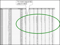
The unusual residual value was identified as corresponding to one particular history from wheel-motor 5509R, with beginning event at 48900 hrs and EF (ending with failure) event at 72005 hrs.The ‘offending’ data is shown in Figure 8
Figure 8 Investigating the strangeness
The Fe values in the left-circled region of Figure 8 have an inexplicable pattern. Fe jumps to high values (but truncated at 2500 PPM due to instrument saturation) and remains in the same range for a few more inspections. Then, the readings fall back to low values. No failure or maintenance events were recorded to explain these sudden jumps.
Having no event data to support such high values of Fe and Si, the offending history was removed from the working data set, and, the model was regenerated. This time statistical goodness-of-fit testing procedures and graphical residuals analysis indicated immediate improvement of the model’s fit to the data. The model no longer had to accommodate obviously contradictory and misleading information.
The forgoing describes data problems which were encountered and which were relatively easy to correct using the statistical and graphical tools available in the software.
However a different (and more fundamental) problem occurred regarding the definition of wheel motor failure. These units seldom failed “functionally”. There were few “in-service” failures requiring that a haul truck be removed immediately from operation. Nevertheless a predictive model requires an objective determination that a unit had failed. It was, therefore, necessary to scrutinize the past work order records to distinquish failures from preventive removals. Initially, the tradesman remarks were used for this purpose, such as "High iron in oil sample and high hours, removed and replaced wheel motor." This event was then classified as a “failure”. However, on reviewing the re-builder's report attached to each invoice it became clear that some events initially classified as a failure should be treated as a suspension (a preventive repair). For example: If the gears had been replaced because they failed an ultrasonic test or they were obviously in a failed state then that life-cycle’s ending event should be classed as a failure. But if gears or other major components were replaced simply because it was expedient to do so, or if the unit was only generally rebuilt with no real internal damage (or major expense), then that history’s ending event should be considered a suspension.
With the definition of suspension and of failure thus clarified, a proportional-hazards model was re-built in the software and found to be a “good fit”.
The model includes the effects of regular maintenance intervals (oil changes) at 500 hrs that occurred regularly during most of the histories prior to the changeover to synthetic oil. A model calculated without including the oil change intervals would tend to underestimate predicted failure times. Oil change events are accounted for by defining (in a database table called CovariatesOnEvent table) the values the covariates would attain were an inspection carried immediately following the (minor repair) event. The PHM parameters and transition probabilities are then estimated from this adjusted data. In subsequent calculations we have to take into account that covariates will regularly have their values reduced. Otherwise covariates will reach high values in the calculation process faster than in real data, and thus produce a higher estimated risk of failure than is really the case.
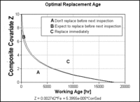
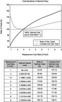
At present the model does not attempt to optimize inspection frequency (a future research feature). Nevertheless, by inspection of the current data on the decision model graph, one would likely choose to increase inspection frequency as the composite covariate (the weighted sum of those variables found to be significant risk factors) approached the boundary condition.It is to be noted (in calculating the benefits of the optimizing model) that no operational savings were accounted for. This was due to the unfavorable coal market conditions at the time, causing the mine to operate below its capacity. As market conditions improve higher cost ratios will be used. Current strip ratios (total material removed versus sellable material) would also affect the savings associated with increased availability and reliability of each haul truck unit. Figure 11 demonstrates the sensitivity of the overall savings to changes or inaccuracies in the cost ratio.
In real situations, the actual ratio of failure and preventive replacement costs may not be well known. Furthermore the dynamics of industry are such that costs can change with changing technology, production, and market conditions. Therefore one should consider how the true total cost (of failure and preventive maintenance when applying the optimal CBM interpretation policy of Figure 10) would change with changes in cost ratio. The software enables sensitivity analysis to be undertaken and generates a graph (Figure 11) and corresponding tabular data.
The curves on the graph are interpreted as follows.
Solid Line: If the actual cost ratio (CR) differs today from that specified when the model was built, that means that the current policy (as dictated by the Optimal Replacement Graph of Figure 10) may no longer be optimal. The line indicates the cost percentage increase that will be incurred (above the optimal cost/unit time for the actual cost ratio) by applying the “optimal” policy (which may no longer be optimal). For example, if the actual cost ratio is 5 and we are using a model which is based on CR=3, then the increase in the cost incurred by following that (now non-optimal) policy is around 6% (5.98). In other words the solid line represents the sensitivity of costs to changes in CR.Dashed Line: Again, assume the actual cost ratio has strayed from what was used when the model was built. If the model is rebuilt using the new ratio the dashed line tells how much the new optimal cost would differ from that of the original model. (Note that the sensitivity graphs assume that only Cf (failure replacement cost) changes and Cr (preventive replacement cost) remains unchanged.) In other words the dashed line represents the sensitivity of the optimal policy to changes in CR. The graph indicates that moderate overestimation of the cost ratio does not significantly affect the average long run cost but provides a more conservative policy from the point of view of risk of failure.
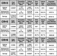
Figure 12 Savings predicted for different economic conditions
Decision model results are also calculated for cost ratios of 5 and 6. As the cost ratio increases we can observe an increase in both the optimal policy cost as well as an increase in savings. The optimal decision models in these cases indicate that more frequent preventive replacements (from 74% to 91%) will result from applying the optimal decision policy. However those preventive actions will avoid a higher proportion of costs due to failure.
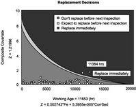
The decision ‘Replace immediately’ was suggested by the model first at working age = 11384 hrs, 286 hours (about two weeks) prior to failure (reported at 11660 hrs). The following inspection (at working age = 11653 hours) 7 hours prior to failure, also recommends the replacement of the wheel motor. The first warning may have been sufficient, given sample turnaround time of 48 hours, to prevent the consequences (high repair cost) of failure. Even prior to 11384 hours it can be seen from the decision graph that the results of the measurements indicate that a replacement recommendation was imminent. The zero points on the graph indicate default measurement values of zero (imputed by the software) immediately following oil changes.
An economic benefit associated with basing the maintenance policy on the Decision Policy Graph (of Figure 10). This investigation indicates a potential saving of between 20%-30% compared to the current practice.
The case study first demonstrates the value of using the technique of PHM to assist maintenance professionals to interpret condition data by identifying the key risk factors and their relative influence on the health of equipment in general, and wheel motors in particular. Economic considerations were then blended with the PHM risk model to identify the optimal decision chart. The study then indicates that the implementation of a condition-based maintenance strategy based on the decision chart would result in a cost reduction of 20%-30%.
Cox, D.R., (1972) “Regression models and life tables (with discussion)”, Jury. Stat. Soc. B, Vol. 34,pp. 187-220.
Jardine, A.K.S., Banjevic D. and Makis V, (1997) “Optimal replacement policy and the structure of software for condition-based maintenance”, Journal of Quality in Maintenance Engineering, Vol. 3, No.2, pp. 109-119.
Campbell, J.D. and Jardine A.K.S. (Editors), (2001) Maintenance Excellence: Optimizing Equipment Life-Cycle Decisions, Marcel Dekker, (Chapter 12: Optimizing Condition Based Maintenance, by M. Wiseman).

