omdec.com

ABSTRACT

This paper describes a case study in which the Weibull Proportional-hazards model is used to determine the optimal replacement policy for a critical item which is subject to vibration monitoring. Such an approach has been used to date in the context of monitoring through oil debris analysis, and this approach is extended in this paper to the vibration monitoring context. The Weibull Proportional-hazards model is reviewed along with the software EXAKT used for optimization. In particular the case considers condition-based maintenance for circulating pumps in a coal wash plant that is part of the SASOL petrochemical company. The condition-based maintenance policy recommended in this study is based on histories collected over a period of 2 years, and is compared with current practice. The policy is validated using data that arose from subsequent operation of the plant.

KEY WORDS: Proportional hazards model, vibration monitoring, optimal replacement policy, case study, circulating pumps

Introduction

The Twistdraai Plant of SASOL, Secunda, South Africa showed preliminary interest in optimizing their condition-based replacement policy. The plant utilizes vibration analysis in maintenance decisions for several types of equipment, such as for circulating pumps. This paper reports development of a condition-based replacement policy based on vibration analysis data and a proportional-hazards model. The software EXAKT was used to produce the results.

EXAKT is software developed in the CBM Lab at the University of Toronto that incorporates the theory discussed above in three main steps: (i) data conversion and preprocessing, (ii) building the statistical and decision model and (iii) making replacement decisions based on current data. In step (i) the data is converted from an existing database as commonly found in EAM’s / CMMS’s (Enterprise Asset Management Systems / Computerized Maintenance Management Systems) to a database suitable for EXAKT. In this process the data quality is checked, data patterns are recognized and additional information required from the user is obtained. See[2] for a detailed overview of the software’s structure.

Some observations on data quality

While analyzing SASOL’s vibration data, several other companies were also visited to investigate the data collection practices and data retrieving mechanisms. Numerous shortcomings were discovered. Some of the major shortcomings are:

(i) Unfriendly or improperly organized CMMS’s.

(ii) Very often, only the calendar age of a component is recorded and not the working age, i.e. the real usage of the component.

(iii) Irregular inspections, sometimes only when maintenance personnel feel they are necessary.

(iv) No records on maintenance done during a component’s lifetime are available.

(v) The state of the item at the time of replacement is seldom recorded, to enable to decide whether a replacement was made preventively or because of failure.

For Proportional-hazards modeling of vibration data to be possible, the data need to fulfil some requirements. From the investigation, a summary of recommendations for future data collection is presented.

Identifying appropriate data

The item must be important enough for periodic diagnostic data collection, i.e. vibration measurements should be taken preferably at fixed intervals. The specific item must have been replaced on a number of occasions in the past, either because of failure or preventively. Data cannot be used for estimation until a certain amount of failures accumulate. Failure does not necessarily mean a physical shutdown or breakage of the item but any condition where the item is unable to perform according to requirements. All available data, such as preventive replacements and calendar suspensions should be included in the analysis and handled suitably. Otherwise, important information could be lost and produce a biased estimate of the lifetime distribution, such as underestimation of the mean time to failure. It is generally assumed that the item is renewed to the as-good-as-new condition at replacement or reconditioning. If not, this information should also be included.

Data collection start and cutoff dates

The start and cutoff dates must be defined when collecting data. All information surrounding significant events should be collected. Items still in operation at the cutoff date should be included in the data set and treated as calendar suspensions. Items already in operation at the start date can be also included in the data set, if the information on the operational age at that moment is available.

Information to be collected

Two main types of data have to be collected:

(i) The operational age of an item at significant events and the type of significant event.
(ii) Diagnostic information (vibration values) at the significant events.

Calendar age at significant events should be also collected. It improves data quality and helps in data analysis. Significant events mentioned above are any of the following:

(i) Moment when the unit is brought into service.
(ii) Every point where diagnostic information is available.
(iii) Points in time where minor maintenance is done that could affect (usually reduce) covariate values, for example realignment, increased lubrication or balancing. The information on what the covariate values might take at these points should also be included in the data.
(iv) The moment when the unit is removed from service for any reason, such as failure, preventive maintenance, discarding because of age, re-selling etc.
(v) Data collection cutoff point for each unit (calendar suspension).

Summary of SASOL data

SASOL produces liquid fuel out of coal. The data was obtained at SASOL Secunda from their Twistdraai coal wash plant. The data was not perfect according to the data needs outlined above (the main reason for the imperfection being irregular inspections). The coal wash plant was started up in September 1996 and is thus relatively new. The data collection horizon was from September 1st 1996 to November 1st 1998 that gave an analysis interval of 791 days. Subsequent to estimating the model parameters using this data set, a second data set was collected from November 1st 1998 to February 28th 1999. This data set was used to test the model’s performance as if it were used for replacement decisions.

Background

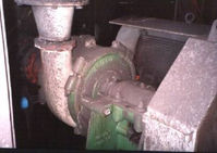
In the plant, 8 identical axial in, radial out pumps (see Figure 1) are used in a specific section of the plant to circulate a water and magnetite solution. All 8 pumps work under the same conditions and can be assumed that the processes of the same type generate all events (failures, replacements, etc) for different pumps. Vibration monitoring is used as a key factor in decisions on preventive replacements of the pumps. Current practice is that no fixed vibration inspection interval is applied from the beginning, but pumps are inspected visually every day. Vibration levels are measured on pumps when there is a visually notable deterioration in a pump’s overall condition, and subsequently more regular vibration inspections are done.

Because of the aggressive nature of the fluid being circulated and the robust environment of the pumps, catastrophic failures are most often encountered. Usually one (or a combination) of the following is defined as a failure:

(a) Complete bearing seizure.
(b) Broken or defective impeller.
(c) Damaged or severely eroded pump housing.
(d) Broken main shaft.

When a pump fails as defined above, it is overhauled completely to an as-good-as-new condition regardless of the amount of work that needs to be done. This may include replacement of bearings, repair or renewal of impeller, repair or renewal of impeller housing or replacement of the main shaft. Sometimes minor grinding is required to the main shaft as well. No complete spare pumps are stocked at the plant but rather spare parts of the total assembly, since some parts tend to fail more often than others.

Figure 1: Circulating Pump

The pumps are driven by 220 kW electric motors via pulleys and V-belts. A shaft runs from the driven pulley to the pump and is supported by two SKF 938 932 bearings. The bearing closer to the pump is referred to as bearing 3 and the other bearing is referred to as bearing 4. The vibration levels on these bearings are measured both in the vertical and horizontal direction and replacement decisions are based on these measurements.

Envelopes or benchmarks are first established for vibration parameters and the pump is replaced as soon as the preset levels are exceeded. Opinion of vibration technicians also played an important role in the replacement decision process because the benchmark levels were primarily based on their experience.

Vibration data loggers were used to do the inspections on the pumps, from where the information was downloaded into E-Monitor, a dedicated computerized vibration measurement database. Data used in this study was retrieved from this database. Frequency spectra of all measurements are stored in the database and the chosen covariate levels (discussed later) could be retrieved easily from it. Failure analysis records obtained from the CMMS provided insight on the state of a pump when it was renewed, i.e. whether it failed or was suspended (preventively replaced). The only other action performed on a pump during its lifetime is additional lubrication that by technicians’ opinion does not effect the vibration levels significantly. This information is not stored in the database.

Data

The data that was collected includes the pump unit identification, dates of inspections, vibration frequency spectrum at each inspection, date of failure or suspension and the state at renewal, i.e. failed or suspended. Inspection data was not available for the cases where unexpected failures occurred and the data was generated by extrapolating available data as appropriately as possible to the date of unexpected failure. This was done more for modeling purposes, not as a required procedure in practice.

A total of 27 pump lifetimes histories were compiled over the analysis horizon with 98 inspections (extrapolations included). This gives an average of 3.6 inspections per history. Approximately 50% of all inspections were done on an irregular basis, either at the beginning or the end of a pump’s lifetime. Of the 27 histories, 11 were failures, 8 were suspensions and 8 were calendar suspensions since all 8 pumps were running at the cutoff date. The 11 failures were all unexpected failures where production losses were suffered. Data shows two groups of failure times: 6 “short” failures (between 75 and 194 days), and 5 “long” failures (between 450 and 563 days). The 8 suspensions were all considerably cheaper preventive renewals based on measured vibration information. Three of the 8 suspensions were done at very short life times relative to other survival times.

The working ages of the pumps are considered to be almost the same as the calendar ages because the pumps run 24 hours per day, except for 10 hours on Sundays, when the plant is out of production due to limitations on production. Very seldom the pumps are shut down because of breakdowns on other parts of the plant and these times are considered to be insignificantly small.

Covariates

Covariates that could be useful in the analysis were selected based on the experience of vibration technicians at the plant. Only the horizontal vibration measurements on two bearings were used and 6 covariates (frequency amplitudes) on each bearing were included. The technicians believe the selected covariates are good indications of an approaching failure. Table 1 below summarizes the covariates, where (3/4)H refers to the horizontal measurement on bearing 3 or 4.

Table 1: Summary of covariates

The reason why the presence of high frequency domain components (HFD(3/4)H) or a lifted noise floor (LNF(3/4)H) was indicated by a ‘0’ or ‘1’ is to include technician’s experience in covariates. When a technician has to estimate the useful remaining life of a pump he simply looks at the presence of high frequency domain components or a lifted noise floor in the frequency spectrum to help him make his decision. The severity of these phenomena is not included in the covariate values but it is possible to add more levels of the severity. Covariates HFD(3/4)H and LNF(3/4)H are referred to as ‘subjective’ covariates.

In a preliminary analysis of the data it was observed that RF1(3/4)H both have a decreasing trend over time. The reason for this is probably because vibration caused by misalignment becomes less and less as the pump wears out. Also, on two occasions, extremely high values for RF043H were observed before suspension. This could be due to manufacturing defects in the specific bearings.

Data modeling results

Weibull PHM fit

There is no straightforward procedure to select the most appropriate covariates for a good Weibull PHM. These procedures are similar to those used in conventional regression analysis. Detailed, non-technical description of model development procedures can be found in[16]. See also[7]. We combined backward selection (eliminating covariates with the highest p-values one at a time), residual graphs, goodness-of-fit tests and technical experience to get to a useful model. Reviewers of this paper suggested that the AIC criterion20 might be useful for model selection as well. Other criteria that could also be useful are Mallow’s C16 and BIC21, recommended for small data sets.

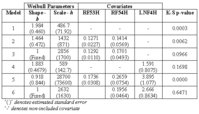
The pump data was analyzed in 4 phases. Each phase is briefly discussed below. The data on estimation for selected models in each category is summarized in Table 2.

Table 2: Summary of estimation for selected PH models

(1) Simple Weibull model (Model #1 in Table 2). The estimate of the shape parameter is 1.984, with a standard error of 0.46, showing it is significantly different from 1. The mean time to failure from the model = 415.5 days, is realistic. The model fit obtained from the K-S goodness-of-fit test has a low p-value, indicating that the age of the pump only cannot explain its lifetime duration.

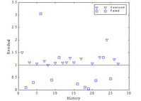
(2) PHM, but ignoring the subjective covariates. After selection procedure, the covariates RF53H and RF54H remained in the model as significant variables (Model #2 in Table 2). The observed p-value is 0.00628. Residual graph is shown in Figure 2 below. This low p-value could be due to that 4 of the 6 “short” failures cannot be well explained by the model, e.g. due to high covariate values. Also, the K-S test value can be affected by the large proportion of suspensions, and the real censoring mechanism applied in the plant. This comment means that K-S test p-value cannot be the only criterion in the selection of the model.

Figure 2: Residuals in order of appearance (Model #2 in Table 2)

It was noticed in all considered models that the shape was not significant. When the models with b=1 were estimated, a better model fit was almost always obtained (Model #2, but with b=1 is referred as Model #3 in Table 2) . This could imply that time (working age) is not a significant variable in the model and that some of the failures could be better explained by an additional non-observed covariate. The vibration technicians do not agree with the statement that time is not significant, and the problem could maybe lie in the lack of data.

(3) PHM, but considering only subjective covariates. The analysis showed that only LNF4H (lack of lubrication on the 4H bearing) could be useful as an indicator of pump problems (Model #4 in Table 2). Even though the value b=1.883 is not significantly different from 1, due to the large standard error, the model with b=1 (not included in Table 2) showed a worse model fit.

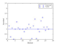
(4) PHM, with all covariates considered. When RF53H, RF54H and LNF4H were included in the model, as would be suggested from step (2) and (3), they appeared as significant, but again with poor test model fit, both for b estimated (Model #5 in Table 2), and for b fixed to 1. The correlation of RF53H and RF54H (about 0.60) might explain why the better model fit was obtained when only RF53H, or RF54H was included in the model. The model with RF54H and LNF4H and b fixed to 1 (Model # 6 in Table 2) has better model fit than other models. From the residuals it appears (see Figure 3 below) that this model could better explain some of short failures than the model without LNF4H. This definitely indicates that subjective covariates could be useful in the pumps’ “health” diagnosis. Some practical questions remain, such as: how much these covariates are subjective, are they convenient for collection, do they differ significantly amongst technicians, etc?

Figure 3: Residuals in order of appearance (Model #6 in Table 1)

From all models discussed in the previous analysis, the model with covariates RF54H and LNF4H, and b fixed to 1 (Model # 6 in Table 2) has the highest p-value, and shows good residual graph. When we presented our analysis and results to the vibration technicians, they suggested to us to consider also the model with covariates RF53H and RF54H (Model #2 in Table 2), because they appreciate these two frequency bands as good predictors of failures. As we see, their experience is consistent with the selection procedure described in (2). Hence, we decided to consider both models in further analysis.

Transition probability matrix

To calculate the optimal policy, we need to calculate the transition probability matrix for selected covariates. Here, we will present part of our results obtained for Model #2. The following covariate states or bands were defined for RF53H: {0-5, 5-10, 10-15, 15-27, 27 and over} and for RF54H: {0-3, 3-7, 7-11, 11-15, 15 and over}. They were selected by combining practical experience and covariate distribution histograms. The software suggested 27 as a reasonably high value for RF53H. With the above covariate bands, the transition rates were determined, and the transition matrix can be calculated for any observation period. For example, the transition probabilities for covariate RF53H at an age greater than or equal to 100 days and an observation interval of 50 days, are given in Table 3.

Table 3: Transition probability matrix for RF53H (current age greater than 100 days and the observation interval of 50 days; row index refers to the current state of RF53H, column index refers to the state of RF53H after 50 days)

From the table we see that if RF53H is, for example, currently between 5 and 10, it will stay there with a probability 48.1%, go up with a probability 31.1%, or go down with a probability 20.8%. This is realistic in practice since vibration levels most often increase with the deterioration process but they can sometimes decrease because of specific wear mechanisms present in the component.

Cost function and optimal replacement policy

To build the final decision model we have tried two models: Model #6, and Model #2. We have tried the second model, even if it did not have a good model fit, as a model more favorable to the technicians. Both models appeared as good decision models, without significant differences in the decision results. The results obtained for Model #2 will be presented in this subsection.

Records show that the average contribution of a pump to production is R 17,150 / hour while a new pump costs R 25,000. (“R” refers to “Rand”, the South African currency). Technicians estimated that a failure replacement takes on average 8 hours to perform. From these figures a cost of failure, Cf, of R 162,200 was determined and R 25,000 for the cost of preventive replacement, Cp. No production is lost during the preventive replacements since they are always done on Sundays, when the plant is not in production. In this study, we will also assume that there is a negligible difference between an immediate preventive replacement and a preventive replacement at the next shutdown, since the next scheduled (“forced”) shutdown is never further than 6 days away, which is also small compared to the average inspection interval. No formal fixed inspection interval was used in the plant to collect data, but for the calculation of the optimal policy a value of 50 days was used, close to the average inspection interval. The resulting cost function , was calculated as a function of the threshold risk level d (for ). This cost function appeared flat about the optimal risk level d*, which means that the optimal policy is relatively insensitive to slight deviations from the decision rule, e.g. to replace slightly after the recommended time.

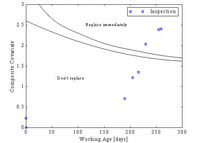
The graph of the calculated optimal replacement policy is given in Figure 4.

Figure 4: Optimal replacement policy

As long as the condition indicator (called the “composite covariate” in the software) at a certain working age falls in the region named “Don’t replace before next inspection” operation should continue. If the condition indicator yields a value that lies in the area called “Replace immediately” instantaneous replacement should take place. The area between these two is a warning region and if the condition indicator lies in this region replacement should take place before the next inspection.The summary of the cost analysis for the theoretical optimal model and the actual SASOL data is given in Table 1. Detailed comments are given below.

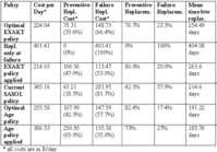
Table 4: Summary of cost analysis 4

The table shows that EXAKT predicts that the average cost of R 224.4 / day would be obtained if the theoretical optimal replacement policy were applied (Optimal EXAKT policy in Table 4), with 66.4% of the costs due to failure replacements. With this policy, still 23.3% of all replacements would be at failure. With a relatively high replacement costs ratio of R 162,200 / R 25,000 = 6.5, such high percentage of failure replacements would be due to the parameter b close to 1, i.e. some random factors not in the control of the maintenance. A reviewer’s suggestion is that it might be also due to small correlation between actual conditions and the condition indicator. The average time between replacements is calculated to be 254.5 days. If no replacement policy were used, except at failures (Replace only at failure in Table 4), it would result in a mean time between failures of 404.1 days, but with the average cost of replacement of R 401.4 / day. This would be 44.2% more expensive than using the optimal EXAKT policy. Using the simple Weibull model estimated from the data (see Model#1 in Table 2), the optimal preventive replacement age is recommended to be 204 days. This policy (Optimal Age policy in Table 4) appears to be theoretically slightly worse (15%) than the optimal EXAKT policy, but this result is doubtful due to bad model fit for the simple Weibull model.

To evaluate the above mentioned theoretical results, we can compare them with: (a) the actual average replacement cost per day realized for the analyzed histories (results included as Current SASOL policy in Table 4), (b) the average replacement cost that is obtained when the EXAKT theoretical optimal policy is applied backwards to the analyzed histories (results included as EXAKT policy applied in Table 4), (c) the cost that is obtained if the optimal age policy is applied backwards to the analyzed histories (results included as Age policy applied in Table 4).

(a) When the current SASOL cost is compared to the EXAKT theoretical optimal cost, the saving would be (345-224)/345 = 35%. The actual policy is slightly better than the policy to replace only at failure, with a saving of (401-345)/401 = 14%.

(b) The optimal EXAKT decision policy was tested using all 27 histories. The number of failures was then reduced from 11 to 4, which is then 4/20 = 20% (temporary suspensions excluded as not decided), close to the theoretical value of 23%. Replacement times were not significantly reduced, which resulted in a (345-214)/345 = 38% reduction of the average cost. The average replacement time is 263.6 days (7 undecided temporary suspensions excluded), close to the theoretical value of 254.5 days.

(c) When the preventive replacement age of 204 days was applied to the historical lifetimes, the number of failures was reduced form 11 to 6. The replacement times were also reduced, and that resulted in a cost/day = R 386.33, significantly bigger (80.5%) than when the optimal EXAKT policy was applied. This also indicates that the model that includes age only is not a good one.

The coincidence of the theoretical and actual results in some of the above cases need not be expected in general, particularly for a small sample size, but here it shows that the selected decision model was reasonable. The method of comparison could be argued because the same data is used to build the model and to test it. The method can be justified by noticing that the data is used to build the statistical model, and then to calculate the optimal decision policy, without referring to the actual replacement policy. Theoretically, the same statistical model would be obtained (within the range of a statistical error), even if the actual policy was to replace only at failure, if the censoring is not informative (i.e. does not anticipate failures). With larger data set (more histories), one could use other methods, such as to use a random sample of histories to build the model, and then the rest as a “control” group.

Example policy

As mentioned earlier, more data was collected between November 1st 1998 and February 28th 1999 to test the optimal policy calculated from the data collected before November 1st. Between November 1st 1998 and February 28th 1999, 2 pumps failed unexpectedly – both shortly after the EXAKT optimal policy would recommend replacement. For the other 6 pumps that did not fail during this time, the EXAKT optimal policy would recommend 1 pump to be replaced on January 31st, and other 5 not to be replaced between November and February. The pump recommended for replacement was still running on February 28th. As an example, the history after November 1st of one of the pumps that failed is shown in Figure 4. This pump was treated in the calculation of the model as a calendar suspension after 192 days of working life. (This was on November 1st 1998). The pump eventually failed 67 days later on January 6th 1999 at an age of 259 days. A total of 5 inspections were done during this time and the covariate values are plotted on the decision policy graph. The policy recommends preventive replacement on December 9th, 28 days before failure, and again on December 31st, 6 days before failure. Figure 4 shows clearly that an expensive unexpected failure could have been prevented if the optimal policy was followed. This test of the EXAKT optimal policy with additional data collected between November 1st 1998 and February 28th 1999 also shows that the policy is useful as a maintenance optimization tool, but more data should be collected for a definite confirmation.

CONCLUSION

The statistical model for circulating pump lifetime that includes vibration-monitoring process was estimated and used to build an optimal replacement decision policy. The study shows that even with some shortcomings in collected data, vibration measurements can be used in proportional-hazards modeling and that a useful decision policy can be obtained. An appropriate practical definition of failure and preventive replacement is required for correct interpretation of observed lifetimes. Thorough analysis combined with prior experience is necessary to select significant variables in the model. The software EXAKT provides a useful tool that can help maintenance engineers organize their data and produce better replacement decisions.
 

We would like to express our sincere gratitude towards SASOL Secunda for their interest in this project, for supplying us with the data and for giving us permission to publish our results. We wish to thank Thampu Joseph, research assistant at the University of Toronto for helping us to compile and document our results. We also wish to thank an anonymous referee whose comments and suggestions helped us to improve the presentation of the paper significantly. The research reported here is partially supported by Materials and Manufacturing Ontario and The Natural Sciences and Engineering Research Council of Canada (under grant #661-215544/98 CRDPJ).

REFERENCES

[1]. Banjevic D, Jardine AKS, Makis V and Ennis M (2001). A control limit policy and software for condition-based maintenance, INFOR 39: 32-50.

[2]. Jardine AKS, Banjevic D and Makis V (1997). Optimal replacement policy and the structure of software for condition-based maintenance, J. Qual. Maint. Eng. 3(2): 109-119.

[3]. Dale, C J (1985). Application of the Proportional Hazards Model in the Reliability Field, Rel. Eng. 10: 1-14.

[4]. Ascher H (1983). Regression analysis of repairable systems reliability. In: Electronic Systems Effectiveness and Life Cycle Costing (J.K. Skwirzynski, Ed.), pp 647-654, Springer-Verlag.

[5]. Davis HT, Campbell K and Schrader RM (1980). Improving the analysis of LWR component failure data, Los Alamos Scientific Laboratory Report, LA-UR, 80-92.

[6]. Jardine AKS and Anderson M (1985). Use of concomitant variables for reliability estimations, Maint. Mngt. Int. 5: 135-140.

[7]. Jardine AKS, Ralston P, Reid N and Stafford J (1989). Proportional hazards analysis of diesel engine failure data. Qual. Reliab. Eng. Int. 5: 207-216.

[8]. Jardine AKS, Anderson PM and Mann DS (1987). Application of the Weibull proportional hazards model to aircraft and marine engine failure data, Qual. Reliab. Eng. 3: 77-82.

[9]. Love CE and Guo R (1991). Using Proportional hazard Modelling in Plant Maintenance, Qual. and Reliab. Eng. Int. 7: 7-17.

[10]. Cox DR (1972). Regression models and life tables (with discussion), J.Roy. Stat. Soc. B34: 187-220, 1972.

[11]. Anderson M, Jardine AKS and Higgins RT (1982). The use of concomitant variables in reliability estimation, Model. Simul. 13: 73-81.

[12]. Kumar D and Klefsjo B (1993). Proportional hazards model: a review. Reliab. Eng. Syst. Safe. 44: 177-188.

[13]. Press WH, Teukolsky SA, Vetterling WT and Flannery B (1994). Numerical Recipes in C, Cambridge University Press: Cambridge.

[14]. Aitkin M and Clayton D (1980). The Fitting of Exponential, Weibull and Extreme Value Distributions to Complex Censored Survival Data using GLIM, Appl. Stat. 29: 156-163.

[15]. Koziol JA (1980). Goodness-of-fit tests for randomly censored data, Biometrika 67: 693-696.

[16]. Hosmer DW and Lemeshow S (1999), Applied Survival Analysis, Wiley: New York.

[17]. Makis V and Jardine AKS (1991). Optimal replacement in the proportional hazards model, INFOR 30: 172-183.

[18]. Christer AH, Wang W and Sharp JM (1997). A state space condition monitoring model for furnace erosion prediction and replacement, Eur. J. Oper. Res. 101: 1-14.

[19]. Basawa IV and Rao P (1980). Statistical Inference for Stochastic Processes. Academic Press: London.

[20]. Sakamoto Y, Ishiguro M and Kitagawa G (1983). Akakie Information Criterion Statistics, Reidel: Boston.21. Schwarz G (1978). Estimating the dimension of a model, Ann. Stat. 6: 461-464.