CBM (Condition Based Maintenance) Expert Systems
A rule-based expert system encapsulates known relationships between CM data and the deterioration in an asset that takes place due to one or more failure modes. An algorithm (known as inference engine) applies the knowledge base to the current set of CM data.
By Daming Lin and Murray Wiseman
Optimal Maintenance Decisions (OMDEC) Inc.Extracted from Chapter 11 of “Reliabiltiy-centered Knowledge”
CBM (Condition Based Maintenance) Decision Making with Expert Systems
Depending on the physics governing a given application, we learned, in Chapter 7. (page 95), that we may choose from a variety of algorithms with which to carry out the signal processing portion of CBM. Decision making, (the third CBM sub-process), proceeds similarly, using one or more of a diverse array of decision support tools. In Chapter 10. Example 1 Creating a decision model (page 127) we developed a CBM decision policy using statistical modeling techniques and software. A decision policy assists maintenance personnel to interpret and act upon a set of condition monitoring (CM) data. Extensive human knowledge and experience may be available with which to build a CBM decision policy. A rule-based expert system encapsulates known relationships between CM data and the deterioration in an asset that takes place due to one or more failure modes. An algorithm (known as an inference engine) applies the knowledge base to the current set of CM data. In this chapter we describe an expert system developed by DLI Engineering[1] called ExpertALERT™.
Figure 11‑1 CBM signal processing and Decision making using an Expert System
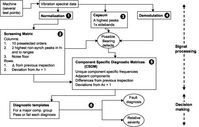
Figure 11‑1 outlines the signal processing and decision making portions of this CBM approach. It traces the flow of information through the signal processing steps (steps 1-5) and the decision making procedure (step 6) that uses a rule-based expert system.
Each machine to be monitored is set up with permanent testpoints[2] positioned strategically (Figure 11‑2) in relation to the components of interest. The equipment is monitored using ExpertALERT™ over a period of time thereby establishing a baseline spectrum for each test point[3] and each orientation. The baseline spectra are updated automatically by the software and set at the average + 1 standard deviation.
Figure 11‑2 An example of test point locations showing the three axes - Axial, Radial, and Tangential
The six steps of Figure 11‑1 are described in each of the following sections.
Step 1 Data normalization
We desire to scale the abcissa of the spectrum in multiples (orders) of the forcing frequency.[4] If the shaft speed is known (from a tachometer signal) the algorithm accomplishes this directly. If it is not known a strong peak is chosen in a window around the nominal speed, or a number of nominal speeds (in the case of a variable speed drive) and the algorithm can successfully match peaks, harmonics and sidebands in order to determine the correct speed for normalizing the spectrum.
The normalization procedure also converts vibration amplitudes to a logarithmic scale in units of VdB. This assists in the visualization of significant, yet low energy peaks, alongside the dominant peaks due to the fundamental forcing frequency. The VdB scale simplifies the interpretation of changes in vibration levels, for example:
- A 6VdB increase = a doubling of vibration amplitude
- A 20 VdB = an increase in vibration amplitude by 10 times.
Next, automated spectral peak extraction and a noise floor calculation are performed. The resulting data populates a “screening matrix”. The columns of the screening matrix represent 10 preselected orders of shaft rate (for example 1x, 2x, ….10x), the two highest non-synchronous peaks in a low and high range spectrum, and a noise floor[5] value.
As an example, let us assume an equipment item has two test points. Then the screening matrix will have (10 orders + 2 peaks x 2 ranges) x 3 orientations x 2 test points + 1 noise floor = 85 columns. One row of the screening matrix will hold the changes in amplitude from the previous inspection. A second row will hold the deviations from the baseline spectrum. A third row will hold the corresponding vibration amplitudes. Hence, in this instance, 85 x 3 rows=255 extracted features will have been placed into the screening matrix, ready for further processing.
The noise floor calculation measures any general increase in random noise. Both impacts and random noise in a time waveform cause the spectrum to become elevated. As bearings wear, they typically produce larger quantities of non-periodic vibration and impacts. This raises the noise floor of the spectrum. The automated diagnostic system uses an algorithm to calculate the level of the noise floor. This value is then compared to a baseline value. Increases in noise floor level add to the severity (see step 6) of the bearing wear diagnosis and may even trigger a diagnosis in certain cases when bearing tones are not evident.
Step 3 Cepstrum analysis
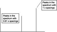
A cepstrum transformation[6] of the fft spectrum is performed next. A cepstrum (Figure 11‑3) highlights series of spectral peaks that are evenly spaced in the spectrum. These are called harmonics Harmonics can be synchronous (multiples of shaft speed) or non-synchronous. The algorithm searches the spectrum for non-synchronous harmonics and any sidebands. If found they are flagged as possible bearing tones, to be processed further in steps 5 and 6.
Figure 11‑3 Cepstrum showing peaks with 1x and 3.61x spacings
Figure 11‑4 Spectrum showing the synchronous and non-synchronous harmonics and their 1x spaced sidebands. The abcissa is scaled in “orders” or mulitples of the shaft speed.
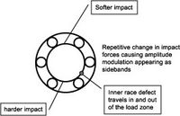
The physics of each situation dictate the signal processing method selected. Non- synchronous peaks, such as those at 3.61 and 7.22 orders (Figure 11‑4), are candidates for “bearing tones” that signal bearing faults. If, in addition, the non-synchronous peaks display sidebands spaced at orders of the shaft speed, an inner race defect is likely. Figure 11‑5 illustrates the physical explanation for bearing tones and the appearance of sidebands, with respect to to an inner race spall or crack.
Figure 11‑5 Physical explanation of non-synchronous peaks and their 1x sidebands related to an inner race spall.
Step 4 Demodulation
Demodulation (also called “envelope detection”) is a signal processing technique used by ExpertALERT to supplement and verify the information drawn from the cepstrum and spectrum analyses. Demodulation provides an independent confirmation of bearing defects.
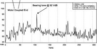
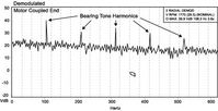
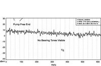
If there is a spall on a bearing race, each time a ball passes it will impact and “ring” the bearing causing it to resonate at high frequencies. The resulting vibrations can be demodulated in order to extract the forcing frequency that is causing the ringing. The forcing frequencies will appear as peaks in the demodulated spectrum. If they match the bearing tones from the screening matrix and the cepstrum, they provide further confirmation of a bearing defect. A distinct advantage of demodulation is that high frequencies do not travel far in a machine. Thus the demodulation process can localize the defective bearing. For example, if you see bearing tones in the narrow band spectral data from two different locations on the machine at the same frequency, and the demod data has matching peaks at one location (but not the other), you can assume that the common location is the one with the bearing problem. The spectra of Figure 11‑6, Figure 11‑7, Figure 11‑8, and Figure 11‑9 illustrate this point precisely.[7]
Figure 11‑6 Spectrum from motor location showing bearing tone peak
Figure 11‑7 Demodulated spectrum from motor location showing matching peak
Figure 11‑8 Spectrum from pump location showing same bearing tone
Figure 11‑9 Demodulated spectrum from pump location, but showing no bearing tones. Hence ExpertALERT can conclude that the bearing defect is on the motor.
Step 5 Component specific diagnostic matrices
The screening matrix is transformed into component specific diagnostic matrices (CSDMs). This transformation extracts values at specific frequencies that characterize possible faults in a given component. It is interesting to note that the techniques of Steps 2, 3, and 4 require no specific knowledge of bearing geometry (e.g. number of rolling elements, inner and outer race diameters, pitch diameter, and so on) for the accurate detection of developing faults. Nevertheless, the CSDM may include specific frequencies based on bearing manufacturing data. Knowledge rules may refer to these frequencies, thus extending diagnostic confidence.
Step 6 Decision making
Steps 1 to 5 may be considered the signal processing portion of ExpertALERT. They extract informative features from the raw vibration data upon which the reasoning engine of the expert system may now operate. Step 6 performs the decision making function, interpreting the extracted features and identifying the likely fault. In Step 6 each CSDM is processed through a series of diagnostic templates consisting of rules that pass or fail every fault known to occur in the component. Furthermore, the expert system computes a score based on the feature’s excedance above the threshold value coded in each rule.[8] The knowledge in the diagnostic templates was developed from an understanding of the physics of the machinery and its causal relationship with the monitored data.
A simple example is the rule for imbalance. This rule checks the matrix elements (of the CSDM) that contain the rotational rate levels and exceedances over baseline. The rule then determines whether these values are are high in a radial direction. If so, other checks determine that the problem is not misalignment or looseness. Finally, the algorithm confirms the imbalance diagnosis.
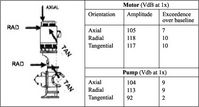
Figure 11‑10 Vertical pump and 1x vibration readings
As an example, consider (for simplicity only the 1x vibration levels of) the vertical motor and centrifugal pump (with coupling), in Figure 11‑10. Excessive 1x vibration may indicate motor imbalance, pump imbalance, angular misalignment, foundation horizontal flexibility, a radial or thrust bearing clearance problem, or motor cooling fan blade damage. Expert system rules based on knowledge of the configuration need to deduce the fault and identify the faulty component.
Looking at the axial and radial data at both locations we might surmise angular misalignment since 1x axial is abnormally high at both motor and pump. Alternatively, it could be motor imbalance or pump imbalance, since 1x radial is abnormally high at either end and radial is higher than axial. Axial motion is, in fact, characteristic (due to rocking) of unbalance in a vertical pump. Another characteristic of a vertical pump is that one direction, the direction of external structural support, is always stiffer than the other directions. The radial axis in this case is the direction of structural flexibility, so that radially, the pump is being “wagged” by the motor imbalance. The low 1x levels at the pump in the tangential direction can be explained by the fact that the tangential axis is the direction of high structural stiffness and therefore the tangential component of the vibration due to motor imbalance does not transmit to the pump.
Rules are activated by machinery component type (for example, in the preceeding, “vertical motor pump set with coupling”) as defined by the user in the ExpertALERT software. A rule for bearing wear in a compressor will look slightly different from the rule for bearing wear in an AC motor. Each individual machine component type may have numerous rules for bearing wear. If the the extracted features satisfy the requirements for a rule, it means the fault condition exists.
After information has been extracted from the spectra as described above in steps 1 to 5, it is passed through all of the rule templates that apply to the general machine type to see if any faults exist. The rules are empirically based on thousands of machine tests collected over more than 20 years and are constantly refined as new information becomes available. If a rule is edited for any reason, the change is run through all past diagnoses to ensure that it does not change any previously correct results.
A typical rule looks something like this in terms of its logic:
- If the sum of the exceedance over baseline of all perceived bearing tones in all three axes and all test points (Cepstrum confirmed) is higher than a threshold, or the sum of the noise floor readings from all spectra has increased over the baseline or alarm by a certain amount, then the rule passes.
- If the sum of the amplitudes of all of the perceived bearing tones exceeds some threshold then the rule passes.
- If none of the perceived bearing tones are above a minimum threshold, the rule does not pass.
- If the sum of the shaft rate harmonics from 16x to 100x are above some value, add to the severity.
- If the noise floor is above some level add to the severity, and if it’s above a higher level, add more to the severity.
- If the sum of the other un-defined peaks that were not confirmed by Cepstrum are above some threshold, add more to the severity.
- If sub harmonics of the shaft rate have exceeded the baseline by a certain amount, add to the severity.
Once a fault has been diagnosed, the user will continue to monitor the machine and look for changes in severity of the fault. The rate at which the severity increases gives a good indication of when the bearings should be overhauled.
The amounts by which the values in the CSDM exceed the threshold values (set up in the rules based on experience and knowledge) is scored and converted into a relative severity. This normalizes a scale with which to judge the state of health of each component. Thus the relative severity for all components in the equipment can be trended on a single graph, as in Figure 11‑11. The graph provides a decision support tool for performing a corrective action on a component whose severity is high or has increased substantially. In the following section, we will propose to extend the automated diagnosis one step further to extimate remaining life and provide an optimized repair decision.
Figure 11‑11 Severity graphs for an equipment item with three components
A proposed hybrid decision tool
Following step 6, the automated diagnostic tools hand over their findings to the human decision makers. Can we process each diagnostic fault and its respective severity one step further to provide:
- A residual life estimate relative to each failure mode, and
- An optimized decision as to whether
ii. to repair within a particular time period from the current time, or
iii. to continue operation until the next inspection. ?
The severity values computed for each fault, as well as the absolute and relative values of the relevant features, may be used as covariates in a proportional hazard model such as that described in Chapter 10. The next section describes the ABB fault simulator that may be use to demonstrate this proposed extension to ExpertALERT’s output report.
The ABB fault simulator
Figure 11‑12 The fault simulator (top left) gradually induces one or more failure modes (for example, misalignment or unbalance). The failure mode (unbalance) causes the failure mechanism (right) to proceed towards failure. The failure is the loss of function to hold the Tee in place by spring friction forces under the stress of vibration forces transmitted through the structure.
In the fault simulator, a spring and friction failure mechanism has been set up with the following characteristics desirable for the study of a failure modeling and prediction methodology.
- A functional failure is clearly defined (by the release of the tee causing the golf ball to trigger a switch).
- The (random variable) time to failure can depend both on working age and CM data.
- A life cycle can be as small as 1 minute, permitting a large sample of life cycles from which to build and subsequently test the predictive model.
How ‘predictive’ can such a model be?
The “goodness” (predictability) of the model depends on two factors:
- How good the data is (its intrinsic information content regarding a progressing failure mode), and
- How big the sample is (the number of life cycles used to build the model).
Figure 11‑13 Running recommendations from the EXAKT agent
Figure 11‑13 displays the running prognostic results that are updated at each inspection. The “Optimal Maintenance Decision” may be one of :
- Continue operation, or
- Plan to replace in a specified number time units, or
- Replace immediately
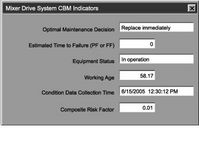
Figure 11‑14 Key CBM performance indicators
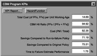
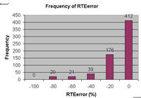
Figure 11‑14 shows the console display of the CBM program KPIs for the demonstration fault simulator unit running an EXAKT optimal decision policy. The predictability of the CBM policy is measurable. It is reflected in the “Time to Failure Estimate Performance”. This figure is the average error in the TRE calculated at each inspection of every life cycle. A histogram (Figure 11‑15) is another way to indicate the predictive performance of the model.
Figure 11‑15 Histogram showing the errors in replacement time estimate over 678 inspections. For example the TRE calculated at 412 inspections were within 5% of the actual (functional or potential) failure time.
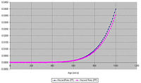
The hazard function curves (in Figure 11‑16) for potential failures and functional failures provides an overall performance check on the effectiveness of the CBM program.
Figure 11‑16 Hazard functions for potential and functional failures
If the difference between TF (total failures) and the FF (functional failures) hazard curves is small, that indicates that the CBM program is effective. That is, functional failures (those that have important consequences) are being preempted by the CBM detection and correction of potential failures (that have none or relatively minor consequences).
Figure 11‑17 ExpertALERT operating on the ABB Asset Optimizer Workplace
Figure 11‑17 illustrates a typical report issued by ExpertALERT. It contains quantitative information relating to the detected fault as well as a recommendation and a “Figure of Merit” indicating the fault severity. The CBM demo links these outputs from ExpertALERT to an EXAKT decision agent. The agent applies a model of the severity ratings and other relevant data extracted and computed by ExpertALERT. The new combined report contains, not only a structured identification and severity rating of the fault, but also an an optimized recommendation including an estime of the time-to-failure.
[2] Testpoints may be equiped with permanent triaxial accelerometers, or a triaxial accelermoter connected to a portable data collector may be used. The barcoded test points must offer a solid screwed mounting for accelerometer.
[4] This simplifies distinguishing the non-synchronous peaks and their sidebands from the dominant forcing shaft frequency and its harmonics. A necessary step in the diagnostic process.
[5] An increase in the noise floor level is an indication of impacting and non-periodic (or random) vibration. Both of these are associated with later stage bearing wear.
[6] One may say in a general sense that the more harmonics and sidebands present, the worse the condition of the bearing. Thus, not only does one wish to know if a peak is part of a larger family of peaks, one also wants to get an idea of how much energy is contained in the series. Cepstrum analysis is used for automating this task. The Cepstrum is a power spectrum of a power spectrum of a waveform; therefore, any periodicities in the spectrum (such as harmonic series or sideband families) will clearly appear as a peak in the Cepstrum.
[7] Alan Friedman, DLI Engineering, Demodulation - June 1999 issue of P/PM
[8] Rule thresholds are a matrix that include both absolute amplitudes as well as exceedences over (mean + 1 sigma) baseline.
