OMDEC - Optimal Maintenance Decisions Inc.

We gather information in the course of our day-to-day maintenance activities in order to deepen our understanding of failure so that we may better manage its causes and control its consequences. We use our growing knowledge of the causes and effects of failure to improve reliability. By "reliability improvement" we mean the attainment of desired levels of availabilty, reliability, operating/maintenance cost, yield, production rate, safety, and environmental integrity of each significant physical asset in its operating context.

How do we achieve any objective in maintenance? Invariably, by adding or altering an aspect of some maintenance policy. Every maintenance department, consciously or unconsciously, operates according to a set of policies. Policies may have been written down explicitly as guidelines and procedures, or they may have originated long ago and persist as habit and tradition. The physical asset manager, in his primary role, monitors the effectiveness of currently active policies. Those polices govern the reliability of the significant items that fall within the compass of his responsibilities.

In the preceding chapter, we described methods and tools for using the CMMS to report the outputs of an existing maintenance policy. For example, the graph of Figure 3-9 (page 41) reports on the effectiveness of our current CBM program. And the graphs of Figure 3-10 (page 42) describe the actual failure behavior of items. They provide clues as to whether a different maintenance policy or physical modification may act to our advantage.All the previous methods help us track the effectiveness - the maintenance outputs - of past and present policies. They do not predict what would happen in the future if a maintenance policy were altered. The capacity to perform “what if” analysis on the future impact of policy changes, would, no doubt, assist the physical asset manager. He could, thereafter, ask questions of the type, “What will the downtime/availabilty/reliability/cost be of my system if I double/triple/halve the overhaul frequency?” We can perform decision analyses such as these by building and running a model. In this chapter we examine the powerful modeling technique known as Monte Carlo Simulation.

Modeling a simple system using SPAR[1]

Assume that we have operated and recorded, in our CMMS, failure and installation events of a simple item over a number of years. We note from these records, that the average life (MTTF) was 0.5 years. We observed the average repair time (MTTR) to be 10 days (0.0274 years) and that the actual repair time was normally distributed with a 10% standard deviation. We desire, at this time, to predict the maintenance performance for this item over the next two years under a variety of alternative policies and conditions.Objective of the analysis

To predict maintenance performance for various failure distributions and maintenance policies:

1. Perfect repair
2. Imperfect repair

1. Various repair effectiveness values
3. Periodic overhaul
1. Perfect repair
2. Imperfect repair

We proceed to build a model by providing SPAR™ with three types of information:

1. the system function (the reliability block diagram) using the Graphical System Function Generator,
2. the failure and repair behavior, using the Input Generator, and
3. the maintenance policies, using the Bubble Logic Generator.

The system function

 

Figure 5‑1 The reliability block diagram for a single line replaceable unit (LRU) named "SGN"Figure 5-1 presents the simplest of reliability block diagrams containing a single line replaceable unit

Failure behaviors

As a hypothetical set of cases for our examination, we will assume 4 possible failure distributions for the single LRU of Figure 1: 1) exponential, and 2) Weibull with shape parameters 1.5, 2.5, and 3.5. An exponential distribution’s single parameter is the item’s MTTF, which in this is case 0.5 years. For the three Weibull distributions, we may calculate the second (scale) parameter, l, using the equation:

Equation 1

where G is the gamma function[2]. And MTTF =0.5. Equation 1 yields the following values for the Weibull scale parameter, l:

Table 1

We can now enter, into the SPAR™ program, the parameters of the 4 failure distributions, and the parameters for the repair time normal distribution (0.0274 years and .00274 years). We specify a service time observation window of 2 years and run the program.

Running the program

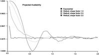
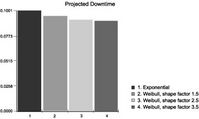
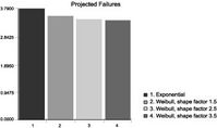
SPAR generates the prediction graphs for availability, downtime, and failure of Figures 2, 3, and 4:

Figure 5‑2 Graphs of predicted availability over 2 years for each of the 4 distributions

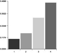
Figure 5‑3 Predicted average downtime over 2 years for each of 4 distributions

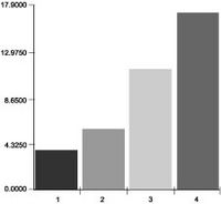
Figure 5‑4 Predicted number of failures in a two year period for each of 4 failure distributions

Remarks

We may conclude that it is technically feasible, (knowing the failure and repair distributions) to analyze and predict maintenance performance. At this point we increase the level of realism one notch by considering policies where repair effectiveness willl be be less than “perfect”.Repair effectiveness

We define “repair effectiveness” as a reduction in age. Following a perfect repair we would “reset” a component’s age to zero. That is, age conservation for a 100% effective maintenance action is “0”. If the repair is imperfect we use the SPAR program’s bubble logic to instruct the calculation engine to conserve a portion of the item’s age after repair. Assume, for example, that a “minimal” repair will actually conserve 99% of an item’s age[3]. We enter this information into SPAR using its Bubble Logic generator tool. SPAR then generates the following Dynamic Logical Sentence (DLS):

Table 2

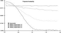
The DLS tells the calculation engine to treat repair as “minimal”. We run the analysis once again. This time, however, the predictive results will account for the minimal nature of the repair. We refer to such repairs as “as bad as old”. Compare the results of the following graphs (Figures 5, 6, and 7) to the previous ones (Figures 2, 3, and 4) where a perfect repair policy was assumed.

Figure 5‑5 Predicted availability under a minimal (“as bad as old”) repair policy

Figure 5‑6 Predicted downtime under a minimal (“as bad as old”) repair policy

Figure 5‑7 Predicted number of failures under a minimal (“as bad as old”) repair policy

We note that the repair policy "as bad as old" leads to lower system performance than in the "as good as new" case. This is expected. However, it is not true (comparing the blue lines and bars of each set of graphs) for the case of an exponential failure distribution. That is because the exponential distribution is "ageless"; a unit whose failure distribution is exponential is always as good as new! At this point we ratchet up the level of realism another notch by adding preventive maintenance (periodic overhauls) to our maintenance policy for this item.

Applying Preventive Maintenance

The purpose of preventive maintenance is to reduce the future chance of unplanned failures, or, in other words, to rejuvenate the component. In this model we shall assume that preventive maintenance reduces the component age back to zero (as good as new). Preventive maintenance is an “external” event that influences the system. We add to our current minor repair policy a proposed preventive maintenance schedule. We do this by using SPAR’s Input Generator tool.

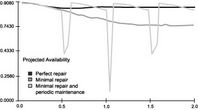
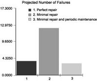
Through a series of dialogs, we modify the current project, by telling SPAR to apply PM periodically at 6 month intervals. We also indicate to SPAR that the PM duration is 14 days (0.0384 years). By default, the PM is considered to apply zero age conservation, which is what we want. As previously, we run the program and generate the maintenance performance prediction graphs of Figures 8, 9, and 10.

Figure 5‑8 Time Dependent Availability for Weibull b=2.5 distribution, (a) Perfect Repair, (b) Minimal Repair, (c) Minimal repair and Periodic Maintenance

Figure 5‑9 Average Downtime for Weibull b=2.5 distribution, (a) Perfect Repair, (b) Minimal Repair, (c) Minimal repair and Periodic Maintenance

Figure 5‑10 Number of Failures for Weibull b=2.5 distribution, (a) Perfect Repair, (b) Minimal Repair, (c) Minimal repair and Periodic Maintenance

Optimizing PM

It is usual to define an optimal PM policy as one that minimizes life cycle cost. Life cycle cost would include the cost of lost production due to failure and maintenance. We set up the variables of our optimization problem as follows:

Table 3

We proceed to determine the optimal maintenance strategy for, say, the case of the Weibull failure distribution with shape factor = 2.5 and a “as bad as old” repair policy. Three possible maintenance strategies are:

1. No maintenance.

2. Preventive maintenance every 6 months.

3. Preventive maintenance every 3 months.

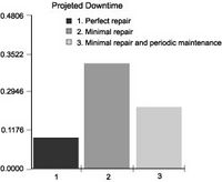
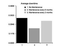
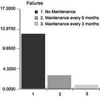
The cases of no maintenance and maintenance every 6 months have already been run. We easily run another case with maintenance every 3 month. Then we have SPAR display the comparative results graphs of Figures 11 and 12.

Figure 5‑11 Average Downtime for Weibull b=2.5 distribution with Minimal Repair and: 1. No Maintenance, 2 Maintenance Every Six Months, and 3. Maintenance Every Three Months

Figure 5‑12 Average number of failures for Weibull b=2.5 distribution with Minimal Repair and: 1. No Maintenance, 2. Maintenance Every Six Months, and 3. Maintenance Every Three Months

Using these results we set up the following spreadsheet calculating cost as Cost = Cd * Td + Cf * Nf + Cm * Nm:

Table 4: Maintenance Policy

On the lower row of this spreadsheet we have applied the following values for this exercise:

Table 5: Variable

We enter the downtimes (from Figure 11) and the number of failures (from Figure 12) into the spreadsheet. The number of PM events (0, 3, and 7) for each case are calculated by hand. (e.g. the number of 3 month interval PMs that will take place in 24 months = 7). We conclude that the most cost effective policy of the three alternatives is to perform preventive maintenance every 3 months. However, a change in the relative costs of failures versus those of maintenance versus those of lost production during downtime will likely change the best policy.

Do you have any comments on this article? If so send them to murray@omdec.com.

[1] Monte Carlo Simulation software availaible from Clockwork Solutions, www.clockworksolutions.com

[2] The value of the gamma function G(x) for any x may be looked up in a table similar to trigonometric tables, for example, sin(x)

[3] For example, to get the equipment back into production quickly, the policy may be to replace only the failed component(s), leaving the others in the unit to continue aging.