omdec.com

By Naaman Gurvitz
Clockwork Solutions

Low failure probabilities are critical factors in business decisions when high costs are incurred due to the consequences of failure. In these circumstances intensive data analysis efforts are employed to assess probabilities of failure. Weibull analysis is commonly used to analyze data, especially in cases where the propensity of failure increases with time and use.

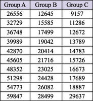
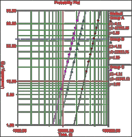
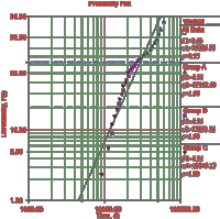
Data analysis techniques and in particular Weibull analyses are very sensitive to the 'mixing of populations', i.e. when operating or environmental conditions that affect the failure rates, are totally ignored or accounted for erroneously in the analysis. In general, the mixing of populations in Weibull analysis will result in an underestimation of the shape parameter. For example, consider three sets of 10 failure times, as listed in Table 1. When analyzing these data sets separately, we obtain three 'perfect' Weibull fits, i.e. each set 'falls' exactly on a unique Weibull line as shown in Figure 1 (with correlation coefficients ρ=1). It should be noted that all three Weibull lines have the same shape parameter (slope) of β = 4.51. If all three sets are analyzed together as a single set, then the best fit is a Weibull line with β = 2.46 (with ρ=0.95) as shown in Figure 2.

In summary, although the population size has increased three times by analyzing the three sets together, the end result is (a) a lower confidence in parameters estimates (i.e. a lower ρ) and (b) a considerable underestimation of the shape parameter (β = 2.46 instead of β = 4.51). The question is: are these consequences of mixing populations important?

Figure 1: Weibull analysis of three individual sets

Figure 2: Weibull analysis with mixing populations

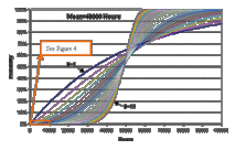
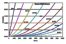
The answer depends on the probability values of interest. But, first it should be noted that Weibull distributions exhibit smaller variance with increasing shape parameters. This phenomenon is especially noticeable in the left-hand tail (or the head) of the Weibull distributions (i.e. for low failure probabilities) as shown in Figures 3 and 4. Figure 3 displays cumulative probability functions CDF[1] of Weibull distributions with the same mean (mean = 48000 hours) but with different shape parameters ranging from β=1 to β=10. Figure 4 focuses on the left-hand side of the same Weibull distributions. So, if the probability values of interest are approximately 50% (or around the mean) then there is no significant difference between Weibull distributions with different shape parameters (as

in cases of sparing[2] in which spares are used for replacement upon failure), but if the focus is on low probability values of 5% or lower (as in cases when preventive maintenance is employed to offset risk and overall cost due to unscheduled failures) then differences in β values are very significant. Underestimation of the shape parameter is equivalent to overestimation of the lower ended probabilities. This overestimation is demonstrated by looking at B1 or B0.5 lives of components. BP life is defined as the time period for which a new component will fail with a probability of P. (For example, the B0.5 life is the time period during which we are 99.5% confident that there will be no failure.) The ratio between a BP life and the mean [3] is independent of the scale parameter or the characteristic life (η) of the distribution. Figure 5 shows a graph of B1 and B0.5 lives to mean ratios as a function of β. Looking at the B1 life curve we can conclude that an underestimation of β=4.51 value to β=2.46 will reduce the B1 time period by approximately 23% of the mean (or a shortening of the time period by approximately 58% compared to the 'actual' B1 period).

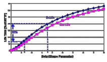
To summarize, failure risk levels (expressed, for example, as B1life) are less sensitive to β at higher β values (Figure 4). The 'mixing of populations' in Weibull analysis tends to underestimate β (Figure 2) and consequently to underestimate B1 life (Figure 5). A robust data analysis methodology that, in effect, 'separates' the entire population to statistically identical subpopulations will result in more accurate and higher β values. This can be accomplished by incorporating covariates in the Weibull analysis. By covariates we mean any type of quantity that affects the failure rates and can be attributed to every observation point, for example, type of fuel, number of starts and so on. Unfortunately in reality covariates vary with time and consequently each observation point is described by a whole 'history' of varying covariate values. This situation is analogous to an attempt to separate balls into groups according to their color while all the balls have many stripes of different colors, and, therefore separation of populations prior to Weibull analysis is simply an impossible task. However incorporating observed covariates values into a Weibull Analysis such as Cox's Proportional Hazard Model, that includes time-dependent covariates, overcomes this problem. With such analysis techniques, a set of 'separated' Weibull curves (as in Figure 1) are obtained [4] rather than a single Weibull curve that includes the entire population (as in Figure 2). This option is viable only if a whole history of covariate values were indeed collected and this information can be attributed to each of the observed time points. Today's data oriented industrial and business environment favors such an extension of reliability analysis.

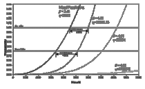
Figure 6: B1 and B0.5 lives (derived from Weibull analysis) with mixed and separated populations

Notes:

[1] CDF, the cumulative distribution function is denoted by F(t) and describes the probability of failure in a time period (ranging from 0 to time t).
[2] It is assumed here, for purposes of illustration, that when spares are available the probability of failure is quite high.
[3] Bp to Mean ratio: where Γ is the Gamma function
[4] Actually what is obtained from analysis are estimates of Weibull distribution parameters η, β and a set of covariates coefficients γ1, γ2, …γn