Table of Contents
Table of Contents
Introduction
-
You may be wondering about the the famous RCM failure patterns or Age-Reliability Characteristics Curves.
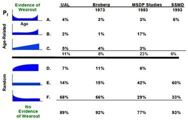
A common question is the following.
“For the 139 items covered by the N&H study, for example, do these curves represent the real failure behaviour of the item? Or do they represent the “effective” net age-reliability relationship (considering that most of these items were subject to time-based maintenance?)”
This is an excellent question. Many maintenance and reliability engineers themselves are not completely sure of the answer nor of its underlying explanation.
Life (Age) Data Analysis
-
Weibull analysis
-
When one carries out so called “actuarial analysis” (more simply referred to as “reliability analysis”) to draw these curves, it is, indeed, to discover the true failure behaviour of an item with respect to each of its significant failure modes, regardless of the maintenance plan currently in force. How is this possible? Are we not basing our analysis on life data from equipment that has been maintained according to the present maintenance strategy and schedule?
The short answer is that at the time of maintenance (say, of the preventive renewal of a component) we will have made certain observations about the state of the maintained items. It is unlikely that we will have observed that all of the renewed items were on the verge of failure. Rather (unless the PM (preventive maintenance) plan is extremely conservative) some items will have failed prior to the moment of PM. (That is, they will have failed in service.) On the other hand, some of the renewed items will not have been in a failed state at the moment of PM. On the contrary, they would have been in excellent condition. Finally, indeed, some items will have well been “on their last legs” and just about to fail functionally. In those cases one might consider PM as being “well timed”.
An astute manager, made aware of the above observations, would undoubtedly ask “what is the optimal moment at which to conduct maintenance”. What PM schedule (termed a policy) will return the greatest benefit, i.e. give us the best overall availability, from a fleet perspective, over the long term? Our manager recognizes that being too conservative would be wasteful causing us to renew many perfectly good components. At the same time, he would not want to us be too liberal by selecting too long a maintenance interval. That would result in an excessive number of failures in service, increasing costs, and lowering overall reliability and availability.
Let us assume the true failure behaviour were as shown below (in the graph of Figure 14 Conditional probability of failure curve for an item that ages - Failure Pattern B ).
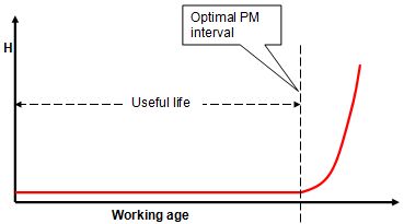
Figure 14 Conditional probability of failure curve for an item that ages - Failure Pattern B
Figure 14 plots the conditional probability of failure[1] against the working age of an item. We would like to be able to claim (to our manager) that our maintenance plan has been optimized. That is to say, that we carry out maintenance at the working age represented by the useful life. Such a strategy would prevent most failures. Yet it would avoid renewal of very many items that are in perfect health. That optimum strategy would issue PM action at a time just prior to a rapid decrease in reliability, termed the useful life.
[1] The conditional probability of failure is the probability of failure in an upcoming relatively short age interval from the perspective of the current moment in time. It is the most important reliability value for daily decision making.
Obviously then, the graph of Figure 14 should represent the inherent designed-in age-reliability relationship of the item if we intend to use it to determine the useful life and, hence, the optimum time based maintenance policy. That brings us to the question, “How to draw this curve, given data from real world, maintained equipment?”
“Real world” implies that our calculations must take into account “suspended” data – data reflecting the actual preventive maintenance programs in place. The most popular statistical method to discover the age reliability relationship is based on the Weibull model for life data. This is an empirical model discovered in the early 1950s by Walodi Weibull, who presented the following equation before an esteemed membership (who reacted with scepticism at first) of the then reliability engineering society.
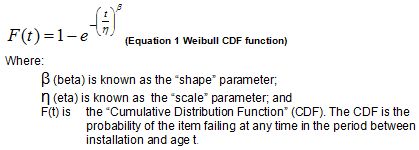
Then we need only determine (estimate from historical data) values for the parameters β and η in order to plot the age reliability relationships. These graphs help us understand the age based failure behaviour of items and their failure modes of interest. Weibull developed a graphical method for estimating the values of the parameters β and η from a set of historical failure data. Today we do not need to use Weibull’s graphical estimation methods. Computerized numerical algorithms based on the Weibull model will estimate the values of β and η and plot the required graphs.
For example, assume we have the following identical[1] items, A, B, C, D, and E and the ages at which they failed.
Table 1:
Item
Failure age
Order[2]
A
67 weeks
1
B
120 weeks
2
C
130 weeks
3
D
220 weeks
4
E
290 weeks
5
The method needs to calculate the corresponding values of the CDF (F(t) in Equation 1) at each of the failure ages 67, 120, 130, 220 and 290 weeks. That is, it must determine a reasonable value for the fraction of the population failing prior to the time of each observation.
[1] A legitimate objection raises the possibility that items A-E may be identical but may operate under varying conditions or duty cycles (harsher or less harsh). The analyst must take this into account by selecting an age measurement other than calendar time. For example: “number of landings”, “number of rounds”, “litres of fuel consumed”, etc. Should variables other than working age be significant, then the Weibull age-reliability model must be extended to include EHM measurements. One such method is described in Annex G.
[2] The “order” is the sequence according to item age at failure.
We cannot simply say that the percentage failed at time 120 weeks is 2/5 because that would imply that the cumulative failure probability at 290 weeks, is 100%. Such a small sample size does not justify such a blanket, definitive statement.
To explain this more clearly, let’s extend the use of the simple fraction to the absurd, by considering a sample size of 1. We would not expect the age of this single failure to represent the age by which 100% of items in the sample’s underlying population would fail. It would certainly be more realistic to regard this single failure age as representing the age by which 50% of the underlying population would fail.
Therefore we need a better way of estimating the CDF, particularly for small samples of lifetimes, in order to apply it to the numerical Weibull solution for plotting the age-reliability relationship. The most popular approach to estimating the CDF from failure data is known as the median rank.[1] A formula, known as “Benard’s probability estimator”, provides an estimate for median rank for small populations, and is given in Equation 2.
[1] For more information on the Median Rank tables and concepts see http://www.omdec.com/wiki/tiki-index.php?page=maintenanceStatistics4.
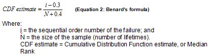
Benard’s formula, applied to our hypothetical single failure, gives (1-0.3)/(1+0.4)=50%, which is intuitively reasonable.
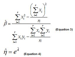
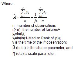
We obtain, either from the median ranks table or from Benard’s approximation, the respective cumulative probabilities of failure (i.e. the CDFs). They are .13, .31, .5, .69, and .87. Of course, when we use reliability analysis software we do not, ourselves, need to look up the median ranks in tables or use Benard’s formula. A computer program applies median ranks automatically to each observation. The algorithm then applies a numerical (regression) technique known as the “Method of Least Squares Estimate” in order to estimate the values of β and η (depicted by their “hatted” symbols) in the following equations:
Suspensions
-
Now that we have discussed, in general terms, the Weibull method for plotting the age-reliability relationship (using historical failure data), we turn our attention to the problem of “suspensions”, which is the main subject of this annex. Let’s begin with the following sample of lifetimes:
Table 2
Item
Failure age
Order
A
84 weeks
1
B
91 weeks
2
C
122 weeks
3
D
274 weeks
4
The items are arranged in sequence according to their survival times. Let N be the total number of observations, in this case, 4, and let “i” be the order (either 1, 2, 3, or 4) of a given failure observation. We can easily apply Benard’s formula to estimate the CDF at each of the four observations. Then we may proceed according to the methods discussed earlier, to determine the Weibull parameters and thus the age-reliability relationship.
But what if item B, for example, did not fail, but was renewed preventively, as directed, say, by the planned maintenance system (PMS) in MASIS? In such a case what would be the order (of failure) i to be applied in Benard's formula? We no longer know the orders of failure because we do not know exactly when (beyond 91 weeks) item B would have failed (had it not been preemptively renewed).
Table 3:
Item
Failure (F#) or Suspension (S#)
Failure or suspension age
Order
A
F1
84 weeks
1
B
S1
91 weeks
?
C
F2
122 weeks
?
D
F3
274 weeks
?
Suspended data is handled by assigning an average order number to each failure time. The table shows that the first failure was at 84 weeks. Then at 91 weeks an item was taken out of service for reasons other than failure. (that is, its life cycle was “suspended”). Two more failures occurred at 122 and 274 weeks.
Had the suspended part been allowed to fail there are three possible scenarios (depending on when Item B might have failed had it not been suspended). In each of these scenarios the hypothetical failure of Item B is denoted by “S1 ->F” in Table 4.
Table 4
Order Scenario
i=1
i=2
i=3
i=4
1
F1
S1-> F
F2
F3
2
F1
F2
S1->F
F3
3
F1
F2
F3
S1->F
The first observed failure (F1) will always be in the first position and have order i=1. However, for the second failure (F2) there are two out of three scenarios in which it can be in position 2 (order number of i=2), and one way that it can be in position 3 (order number of i=3). Thus the average order for the second failure is:

For the third failure there are two ways it can be in position 4 (order number of i=4) and one way it can be in position 3 (order number of i = 3).

We will use these average position values to calculate the median rank from Benard's formula”, as in column 5 of Table 5, for use within Equations 3 and 4.
Table 5:
Item
Failure or Suspension
Failure or suspension age
Order, i
Median rank
A
F
84 weeks
1
0.16
B
S
91 weeks
?
C
F
122 weeks
2.33
0.46
D
F
274 weeks
3.67
0.77
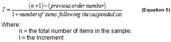
Obviously, finding all the sequences for a mixture of several suspensions and failures and then calculating the average order numbers is a time-consuming process. Fortunately a formula is available for calculating the order numbers. The formula produces what is termed a “new increment”. The new Increment I is given by:
So for failures at 122 weeks and 274 weeks the Increment will be:
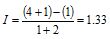
The Increment will remain 1.33 until the next suspension, where it will be recalculated and used for the subsequent failures. This process is repeated for each set of failures following each set of suspensions. The order number of each failure is obtained by adding the “increment” of that failure to the order number of the previous failure. For example referring to Table 5, acknowledge that the Order of Item C (2.33) is indeed 1+1.33, and the Order of Item D (3.67) is indeed approximately 2.33+1.33.
Now that we have calculated the orders i for each of the failure observations, we may use those values to estimate β and η (from Equations 3 and 4).
Although the foregoing seems rather complicated, the availability of powerful reliability software packages renders the job quite easy. For example, Reliasoft’s tool, SimuMatic, requires the user merely to enter or import the data and select the desired calculation method from the dialog (see Figure 15).
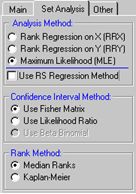
Figure 15 Analysis selection dialog - SimuMatic
Figure 15 implies that there are several alternative calculation methods that can be used to estimate the age-reliability relationship. This annex has briefly described one of them, the Method of Least Squares Estimation with median ranking. Another popular method is known as Maximum Likelihood Estimation (MLE)[1]. This annex has attempted to provide the reader with some insight into the famous RCM failure patterns (Figure 3 on page 14), and, into the question, “How to get the true age-reliability relationship, from real world samples containing suspended lifetimes?”.
[1] For more information on MLE see http://www.omdec.com/wiki/tiki-index.php?page=maintenanceStatistics4
-
Optimizing TBM - cost model
-
Having understood from the above development the method for plotting the age reliability relationship, a practical question comes to mind. We may ask, quite legitimately, how knowledge of the age-reliability relationship can assist in optimizing the maintenance decision process? The following development addresses this important question.
Two additional useful ways to express the age-reliability relationship are as a:
- hazard function [1], h(t)
- This was the form used in the famous six RCM failure patterns (A-F) of Figure 7 . Or as a
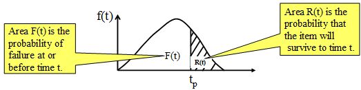
- probability density function, f(t)
- This form has some revealing visual characteristics as follows:
[1] The hazard function is also known as the “failure rate function” or, roughly, the “conditional probability of failure”. It is the probability of failure in the forthcoming relatively short interval of time, given that the item has survived to the start of that interval. An amusing story about the hazard function told by John Moubray can be found in this forum post.
Now let us assume that tp is the time at which, as a policy, time based renewal, is carried out. The obvious question then is, “what should tp be so that it is optimal?”. By optimal, we mean that the organizational objective, say lowest operational cost[1], is achieved. Let's try to answer the question.
Equations 1, 2, and 3 below articulate (and resolve) the problem.
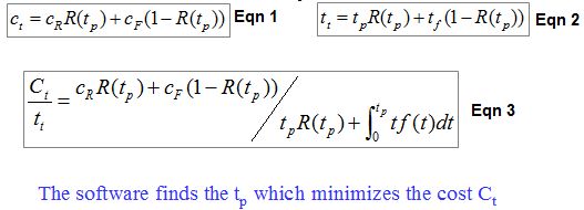
Equation 1 reads as follows:
The expected operational cost, for the average life cycle, ct, is equal to the cost of a preventive repair cR multiplied by the probability that the item will survive until tp, plus the cost of a failure induced repair cF multiplied by the probability that the item will not survive until tp.
[1] The objective could as well equally be specified as “highest possible availability”. A more complex objective function could specify an optimal mix of high availability and high “effective” reliability under the constraints of an upper limit on the life cycle cost.
A similar statement can be made for the expected time of actual maintenance, tt.
The Navy is often interested in minimizing the overall expected cost of maintaining and repairing an item per unit of its working age. This is expressed as a ratio, ct/tt, in Eqn. 3.
It is, in fact a way of expressing “Life cycle cost” of an item related to a “unit” of its usage. Equation 3 can be “solved” numerically for the value of tp which minimizes average life cycle cost.
-
CBM Data Analysis and Prediction
-
Summary
-
This annex extends the principles of Annex F "Life (Age) Data Analysis", to the case where extra information, known as EHM data, is available to further support the maintenance decision process. EHM empowers a maintenance manager to use both working age and monitored variables (such as acoustic and thermal emission, vibration, temperatures, pressures, wear particles, oil contamination, and limitless process data) in order to make informed decisions about whether, when, how, and what to maintain.
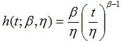
Recalling the development of Annex F, how may we apply a similar rigorous methodology to convert EHM data and age data into optimal maintenance decisions? The Weibull model of Annex F was given as a CDF (cumulative distribution function). It may be rewritten[1] in terms of the hazard function, h(t), as follows:
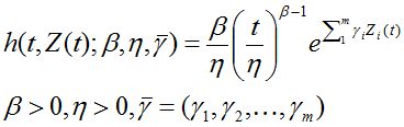
This annex introduces two theoretical models. The first, called the Cox PHM (proportional hazard model), extends the Weibull model to include time varying EHM variables, as follows:
[1] We can convert easily among the functions f(t), h(t), F(t) and R(t) by using the relationships F(t)= 1-R(t), h(t)= f(t)/R(t), f(t)=dF(t)/dt.
Note that only the difference between the Weibull model and the Cox Proportional Hazard Model (PHM) is the factor, e raised to the sum of EHM indicators each multiplied by its respective parameter γi.
Now, using the Cox extension of the Weibull model (called PHM with Weibull baseline), we will model the failure behavior of the item not only as as a function of age but also as a function of relevant EHM variables. We use estimation methods (analogous to the numeric techniques mentioned in Annex F) not only to determine the parameters β and η, but also the parameter vector γ.
In addition to the Cox PHM, in this Annex, we make use of a second model, known as the "non-homogeneous Markov failure time process". It models the probability of transition of the vector of EHM variables from one state to another. This model can be clearly depicted as a transition probability matrix. Such a matrix is readily available from past historical EHM data. For example, considering past values of say, temperature and pressure in, say, a nitrogen compressor, the following (Markov chain transition) probabilities of Table 1 can be calculated:
Table 1: Transition probability matrix
T,P FutureT,PCurrent
1,1
1,2
1,3
2,1
2,2
2,3
3,1
3,2
3,3
1,1
.467
.176
2e-4
.162
.188
3.2e-3
2.5e-4
2.7e-3
0
1,2
.42
.184
2.4e-4
.16
.23
5e-3
3e-4
3.8e-3
0
1,3
.36
.178
7.7e-4
.16
.268
.029
3e-4
4.4e-3
0
2,1
.409
.167
2.2e-4
.183
.232
4.8e-3
3.6e-4
3.9e-3
0
2,2
.35
.175
2.9e-4
.18
.282
7.8e-3
4e-4
5.3e-3
0
2,3
.26
.164
1.6e-3
.16
.334
.066
4e-4
5.8e-3
0
3,1
.338
.163
2.5e-4
.19
.291
6.4e-3
1.5e-3
1.3e-2
0
3,2
.31
.171
2.9e-4
.188
.32
8.2e-3
1.2e-3
1.2e-2
0
3,3
0
0
0
0
0
0
0
0
1
Each of the two monitored variables (gas temperature in compressor stage 3 and pressure in compressor stage 2) has been assigned 3 states - 1, 2, and 3, representing, say, “normal”, “marginal”, and “critical” operation respectively. The pairs (1,1), (1,2), ... in column 1 list all combinations of temperature and pressure at the current moment. Similarly the combination pairs of row 1 represent the all possible future (e.g. say five hours from now) states.
Each cell contains the probability (calculated from past transitions), of movement between any two states, in a prescribed observation interval of, 5 hours. If the current state of temperature and pressure is (1,1), then the probability of remaining in that state 5 hours hence is 46.7%. The probability of transiting to state (1,2) from state (1,1) is 17.6%, and so on.
Table 1 displays a reduced version of the transition probabilities used in the numerical example given at the end of this annex.
The following optional section contains the formal development of the theory behind EHM optimization based on the Cox PHM and Markov failure time process models. It is not necessary to follow the mathematics. Suffice it to say that by combining the Cox and Markov models we may project the reliability forward based upon current working age and the current state of the EHM variables.
This projected survivability is known as the "conditional reliability" function, from which we may calculate the RUL (remaining useful life). Just as we introduced the optimal age-based maintenance decisions policies in Annex F, we now introduce optimized EHM data interpretation models. A numerical example at the end of this annex illustrates the methodology. You may skip the six mathematical sections that follow and go immediately to the numerical example.
Mathematical development (optional)
-
Intro
-
The advantage of EHM over TBM (time or age based maintenance) as a maintenance strategy is that it accounts for both the age of the item as well as its changing state up until the moment of decision making. We assume the item's state of health to be encoded within measurable condition indicators (which, of course, is the underlying premise of EHM).
The item's monitored indicators may be presented as a vector of time dependent random variables, Z(t).
Z(t) = (Z1(t),Z2(t), ... ,Zm(t))(eq. 1)
Each variable in the vector contains the value of a certain measurement at that moment. We considerZ(t) a "process" because it changes with each set of EHM readings acquired at regular intervals of time t. Furthermore, it is a stochastic process. A stochastic process is sometimes called a random process. Unlike a deterministic process, instead of having only one possible 'reality' of how the process might evolve with time, in a stochastic process there is some indeterminacy in its future evolution. This uncertainty is described by probability distributions. There are many possibilities of where the process might go, but some paths are more probable than others. Z(t), then, is said to be an "m-dimensional stochastic covariate process'' observed at regular intervals of time, t.We let T, a random variable, represent the failure time of the item. A primary goal of EHM is to predict T given the current age t and the current measurements of Z(t). Achieving this goal will require us to develop a statistical model that combines the stochastic behavior of the CBM readings Z(t) with a model for the hazard rate as a function of age t and the current CBM readings Z(t).
Of particular interest to us in accomplishing this objective are the two theoretical models alluded to in the summary. They are:-
the Cox proportional hazards model (PHM) with time-dependent covariates for describing the failure behavior, and
- the non-homogeneous Markov failure time process for describing the evolution behavior of the covariate process.
The next section (called "Mathematical development") is optional reading. It shows, in a formal way, how these two models may be combined for the predictive purposes of EHM.
-
the Cox proportional hazards model (PHM) with time-dependent covariates for describing the failure behavior, and
Proportional hazards model with time-dependent covariates
-
The influence of condition monitoring (CM) indicators on the failure time is modeled using a Proportional Hazards Model (PHM). First proposed by Cox in 1973 (Cox D.R., Oakes D., 1984.), the Cox PHM and its variants have become one of the most widely used tools in the statistical analysis of lifetime data in biomedical sciences and in reliability. The specific model to be discussed in this annex is a PHM with time-dependent covariates and a Weibull baseline hazard. It is described by the hazard function
where β>0 is the shape parameter, η>0 is the scale parameter, and γ =( γ1,γ2,… γm,) is the coefficient vector for the condition monitoring variable (covariate) vector. The parameters β, η, and γ, will need to be estimated in the numerical solution.
Markov failure time process
-
The physical CBM measurements of each Zi(t) will fall into classes or states that we have set up and labeled as, for example, "new", "normal", "warning", or "danger". These designations (a common practice in EHM) constitute the state space of the stochastic process Z(t). As such, the covariate vector Z(t) can be reasonably discretized to reflect, meaningfully, each of its states. Specifically, we discretize the range of each covariate Zi(t) into a finite number of intervals each of which has a representative value. This value can be taken as any value in an interval’s range. In this annex we take the midpoint of each interval as the value representing the condition indicator’s state.
Define the discretized covariate process Z(t) as Z(d)(t) = (Z1(d)(t), Z2(d)(t), ... , Zm(d)(t)).
such that the value of each Zi(d)(t) is equal to the representative value of the interval into which Zi(t) falls.Denote all possible values (states) of Z(d)(t) as R1(z), R2(z), …, Rn(z)
where Ri(z) = (Ri1(z), Ri2(z), …, Rim(z)) is a representative value of the covariate Zj(d)(t).
Ri(z) represents the ith state of the discretized covariate process Z(d)(t).
We predict likely future states of the discretized process Z(d) (t), by endowing it with some kind of probabilistic behavior. A non-homogeneous discrete Markov process has been shown (Bogdanoff & Kozin, 1985; Kopnov & Kanajev, 1994; Pulkkinen, 1991) to model the stochastic behavior of time dependent condition monitoring variables related to wear propagation.In this annex we will assume that Z(d)(t) follows a non-homogeneous Markov failure time model described by the transition probabilities
Lij(x,t)=P(T>t, Z(d)(t)= Rj(z)|T>x, Z(d)(x)= Ri(z)) (eq. 3)
where:
x is the current working age,
t (t > x) is a future working age, and
i and j are the states of the covariates at x and t respectively.
Lij(x,t) is the transition probability from state i to state j and can be read as follows: It is the probability that the item survives until t at which time the state of Z(d)(t) is j, given that the item will have survived until x when the previous state, Z(d)(x) was i. The transition behavior can then be displayed in a Markov chain transition probability matrix, for example, that of Table 1.
Table 1: Transition probability matrix
T,P FutureT,PCurrent
1,1
1,2
1,3
2,1
2,2
2,3
3,1
3,2
3,3
1,1
.467
.176
2e-4
.162
.188
3.2e-3
2.5e-4
2.7e-3
0
1,2
.42
.184
2.4e-4
.16
.23
5e-3
3e-4
3.8e-3
0
1,3
.36
.178
7.7e-4
.16
.268
.029
3e-4
4.4e-3
0
2,1
.409
.167
2.2e-4
.183
.232
4.8e-3
3.6e-4
3.9e-3
0
2,2
.35
.175
2.9e-4
.18
.282
7.8e-3
4e-4
5.3e-3
0
2,3
.26
.164
1.6e-3
.16
.334
.066
4e-4
5.8e-3
0
3,1
.338
.163
2.5e-4
.19
.291
6.4e-3
1.5e-3
1.3e-2
0
3,2
.31
.171
2.9e-4
.188
.32
8.2e-3
1.2e-3
1.2e-2
0
3,3
0
0
0
0
0
0
0
0
1
Table 1 displays a reduced version of the transition probabilities used in the numerical example given below.Each of the two covariates (gas temperature in compressor stage 3 and pressure in compressor stage 2) has been assigned 3 states representing, say, “normal”, “marginal”, and “critical” operation. We may examine the likelihood, based on past behavior, of movement between any two states, in a prescribed observation interval of, say, 5 hours. If the current state of temperature and pressure is (1,1), then the probability of remaining in that state 5 hours hence is 46.7%. The probability of transiting to state (1,2) from state (1,1) is 17.6%, and so on.
Calculation of the transition probabilities
-
We now combine the Cox PHM with the Markov failure time model described above. For the following analysis it is convenient to represent Equation 3 in the following form:
Lij(x,t)=P(T>t|T>x, Z(d)(x)= Ri(z))) • pij(x,t) (eq. 4)
where pij(x,t)=P(Z(d)(t)= Rj(z)| T>t, Z(d)(x)= Ri(z)) (eq. 5)
is the conditional transition probability of the process Z(d)(t).-
Lij(x,t)=P(T>t|T>x, Z(d)(x)= Ri(z))) • pij(x,t)
Beginning with equation 3:
Lij(x,t)=P(T>t, Z(d)(t)= Rj(z)|T>x, Z(d)(x)= Ri(z))
make the following temporary substitutions:
a: T>t
b: Z(d)(t)= Rj(z)
c: T>x
d: Z(d)(x)= Ri(z))
Then equation 3 becomes:
Lij(x,t)= P(b,a|c,d)
From the definition of conditional probability, P(e,f)= P(e)P(f|e), we can rewrite equation 3 as:
Lij(x,t)=P(a|c,d)(b|a,c,d)
Since T>t implies T>x
Lij(x,t)=P(b|a,d)P(a|c,d) yielding equation 4.
For a short interval of time, values of transition probabilities can be approximated as:
Lij(x,x+Δx)=(1-h(x,Ri(z))Δx) • pij(x,x+ Δx) (eq. 6)
Equation 6 means that we can, in small steps, calculate the future probabilities for the state of the covariate process Z(d)(t). Using the hazard calculated (from Equation 2) at each successive state we determine the transition probabilities for the next small increment in time, from which we again calculate the hazard, and so on.-
Lij(x,x+Δx)=(1-h(x,Ri(z))Δx) • pij(x,x+ Δx)
Beginning with equation 4
Lij(x,t)=P(T>t|T>x, Z(d)(x)= Ri(z))) • pij(x,t)
For time t=x+Δx
Lij(x,x+ Δx)=P(T>x+Δx|T>x, Z(d)(x)= Ri(z)) • pij(x,x+Δx) (eq. 1A)
Introduce the conditional hazard rate function defined as:
This obviously leads to
1-h(t|Z)Δt=P(T>t+ Δt|T>t,Z)
Substituting this into (eq. 1A) above yields equation 6.
-
EHM decisions based on probability
-
The “conditional reliability” is the probability of survival to t given that
- failure has not occurred prior to the current time x, and
-
CM variables at current time x are Ri(z)
The conditional reliability function can be expressed as:
Equation 7 points out that the conditional reliability is equal to the sum of the conditional transition probabilities from state i to all possible states. Once the conditional reliability function is calculated we can obtain the conditional density from its derivative. We can also find the conditional expectation of T - t, termed the remaining useful life (RUL), as (eq. 7)
In addition, the conditional probability of failure in a short period of time Δt can be found as (eq. 8)
P(tZ(d)(t))=1-R(t+ Δt|t,Z(d)(t)) (eq. 9)
For a maintenance engineer, predictive information based on current CM data, such as RUL and probability of failure in a future time period, can be valuable for risk assessment and planning maintenance.
EHM decisions based on economics and probability
-
The Navy confronted with a variety of requirements and risk factors, seeks to optimize its policies and resources in order to achieve its ultimate objectives. An economic decision model is a rule for preventive renewal of an asset that minimizes the average per unit cost associated with maintenance (proactive and reactive) over a long time horizon. (This cost is the key performance indicator most directly related to taxpayer value.) Such a rule for EHM may be reasonably expressed as a control-limit policy: perform preventive maintenance at Td, if Td <T; or perform reactive maintenance at T if Td ≥ T, where
Td=inf{t≥0:Kh(t,Z(d)(t))≥d} (eq. 10)
K is the cost penalty associated with functional failure, h(t,Z(d)(t) is the hazard, and d (> 0) is the risk control limit for performing preventive maintenance. Here risk is defined as the functional failure cost penalty K times the hazard rate.-
Td=inf{t≥0:Kh(t,Z(d)(t))≥d}
inf{} is the Infimum. Inf{A:B} means the highest value possible that is less than or equal to all the values in A satisfying constraint B.
Therefore, Equation 10,
Td=inf{t≥0:Kh(t,Z(t))≥d}
defines a renewal time Td as the greatest lower bound of all t where risk exceeds the control limit d.
Or, in other words, the equation defines Td as the greatest possible renewal age that is less than or equal to any t for which the risk would exceed control limit d.
The long-run expected cost of maintenance (preventive and reactive) per unit of working age will be
where Cp is the cost of preventive maintenance, Cf = Cp+K is the cost of reactive maintenance, Q(d)=P(Td≥T) is the probability of failure prior to a preventive action, W(d)=E(min{Td,T}) is the expected time of maintenance (preventive or reactive). eq. 11)
-
The expected per unit cost would be the sum of two terms:
eq. 11)
- the cost of a preventive action times the probability (1-Q) that the item will survive long enough for the preventive cost to be spent. So this first term will be Cp(1-Q).
- the cost of a functional failure times the probability Q that the functional failure occurred. So this second term will be CfQ
Divide the sum of these terms by the expected uptime, W, in order to get the cost per unit of working age.
Φ(d)= (Cp(1-Q)+CfQ)/W
Substituting from Cf=Cp+K yields Equation 11
Let d* be the value of d that minimizes the right-hand side of Equation 11. It corresponds to T* = Td*. Makis and Jardine in ref. 3 have shown that for a non-decreasing hazard function h(t,Z(d)(t), rule T* is the best possible replacement policy (ref. 4).
Equation 10 can be re-written for the optimal control limit policy as:
T*=Td*=inf{t≥0:Kh(t,Z(d)(t))≥d*} (eq. 12)For the PHM model with Weibull baseline distribution, it can be interpreted as (ref. 2)
where (eq. 13)
Ref. 2 mentions the numerical solution to Equation 13, which is described in detail in (Ref. 7) and (Ref. 8). The function (eq. 14)
g(t)=δ*-(β-1)ln(t) (eq. 15)
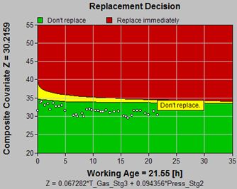
is the “warning level” function for the condition of the item reflected by a weighted sum of current values of the significant CM variables (covariates). A plot of function versus working age can be viewed as an economical decision chart which shows whether the data suggests that the item has to be replaced. In the decision chart, we approximate the value of by
by 
An example of a decision chart with several inspection points can be found in Figure 3. Detailed case studies based on the model discussed in this section can be found in ref. 5 and (ref. 6).
Figure 3: Sample economical decision chart (for β>1)
The above development from (ref. 2) speaks to cost as the optimizing objective. Analogous developments have been made in EXAKT considering availability and profitability as optimizing objectives. For these two objectives, we only need to change the objective function in Equation 11 accordingly.
Specifically, for the availability objective, Equation 11 will be replaced by the availability function, defined as the ratio of uptime to the uptime plus the downtime
where W(d) is the expected uptime, tp is the downtime as a result of planned maintenance and tf is the downtime as a result of maintenance forced by a functional failure. The objective is also changed to maximize (eq. 16)
 , i.e., d* will be the value of d that minimizes the right-hand side of Equation 16.
For the profitability objective, Equation 11 will be replaced by the global cost function
where ap is the cost per hour of planned down time and af is the cost per hour of unplanned down time. The objective is to minimize Equation 17, i.e., to find d*, which is the value of d that minimizes the right-hand side of Equation 17. (eq. 17)
-
-
Numerical example
-
A EHM program on a fleet of Nitrogen compressors monitors the failure mode “second stage piston ring failure”. Real time data from sensors and process computers are collected in a PI historian. Work orders record the as-found state of the rings at maintenance.
In the following example, four decisions are generated by software depending on which of: probability alone, cost, availability, or profitability (cost and availability) has been set as the optimizing objective. The data for this example is available by contacting NETE. Background information on this example and the failure mode can be found in (ref. 9).
Decision based on probability
-
RUL = 106.99616, StdDev = 67.173893
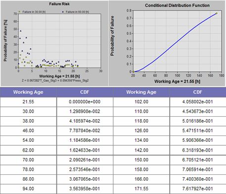
The CDF (Conditional Distribution Function) is the probability of failing between now (the moment of the most recent EHM data) and some specified time in the future. Hence the probability of failure within the next 86 working age units is 30.7%, within the next 171 working age units, 76.2%. The remaining useful life (RUL) is, by definition, the “conditional” mean-time-to-failure. Otherwise stated, it is the mean-time-to-failure counted from the present, based on the current of working age and the values of the observed significant EHM variables.
Decisions based on economics and probability
-
Cost minimization
-
Cost Prev. Cost Failure Cost Preventive
%Expected MTBF
(PF or F)Optimal 29.5473 16.0089
(54.2 % )13.5384
(45.8 % )87.6 54.7487 RTF 48.3946 0
(0.0 % )48.3946
(100 % 00.0 123.981 Saving 18.8473
(38.9 % )-16.0089 34.8562 -83.5 -69.232 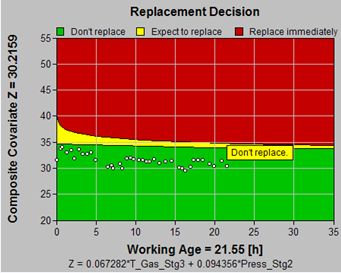
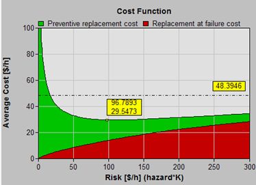
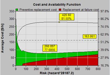
Input Parameters Replacement Policy Type Basic Cost Preventive Replacement cost C $ 1000 Failure Replacement cost C+K $ 6000 Inspection Interval h 30 Decision Parameters Recommendation Don’t maintain Expect to replace in 39.794 Any cost value on the Cost Function graph consists of a red portion, attributable to unplanned failures, and a green portion, representing the average costs associated with preventive maintenance.
The green curve determines the optimal risk as its lowest point (96.7893). The table beneath the Cost Function graph summarizes the information. It compares the optimal cost ($30) and optimal mean time between asset renewals (55 h)) of the optimal policy with those ($48 and 124 h) of the "run-to-failure" policy. It quantifies the expected preventive and failure costs ($16 and $14 respectively) and the percentage of incidences (87.6% will be preventive actions while 12.4% will be failures) achieved when adhering to the optimal policy.
The table's content illustrates that the optimal policy will cause us to intervene more often on the average (every 124 versus 55 h), in order to achieve a net per unit saving (of $19 or 39%).
Availability maximization
-
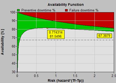
Availability
%Prev.
downtimeFailure
downtimePreventive
%Expected MTBF
(PF or F)Optimal
81.55
(46.93*)9.54
(51.68 % )8.91
(48.32 % )91.5
57.5433
(10.6169**)RTF
67.39
(123.98*)0
(0.0 % )32.61
(100 % 00.0
183.981
Saving
14.16
-9.54
23.70
-91.5
-126.437
Input Parameters
Replacement Policy Type
Basic Availability
Preventive downtime Tp h
60
Failure downtime Tf h
60
Inspection Interval h
30
Decision Parameters
Recommendation
Don’t maintain
Expect to replace in
33.3742
The analyst must supply the parameters of this strategy, which are the fixed values for the downtimes incurred by: 1. preventive renewal (maintenance), and 2. renewal as a result of failure. The costs of materials and labor are not considered significant in this option, or they are believed to be proportional to downtimes and, thus, can be ignored.
This example illustrates the trade-off made in optimizing for availability. In the minimum cost model, above, we "bought" lower overall cost by "paying" for it with more frequent intervention. We assumed that the time-to-repair was negligible, or was proportional to the cost, and therefore could be ignored. The difference between failure and preventive repair costs dictated the exact nature of the compromise in order that overall impact on the per unit production cost be minimum.
In a symmetrical way, the maximium availability model focuses completely on downtime. In this example, we "bought" high availability by paying for it with more frequent intervention. We assumed that the cost of repair was negligible, or was proportional to the repair time and therefore could be ignored. The difference between failure and preventive repair times (rather than costs) dictated the exact nature of the compromise to achieve high equipment availability. The optimal strategy maximizes expected availability per unit time (defined as 100%*uptime/(uptime+downtime)).
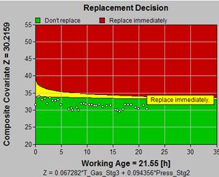
Maximum cost effectiveness
-
Unit cost
AvailabilityPrev. cost
DowntimeFailure cost
DowntimePrev. %
Expected MTBF
(PF or FF)Optimal
77.6856
81.16 (37.33*)45 (58.5 % )
12.40 (65.80 % )32 (41.5 % )
6.44 (34.20 % )95.1
45.9968
(8.66753**)RTF
163.061
67.39 (123.98*)0 (0.0 % )
0 (0.0 % )1.6e+002 (100.0 % )
32.61 (100.0 % )0.0
183.981
(60**)Saving
85.38 (52.4 % )
13.77-45
-12.401.3e+002
26.17-95.1
-137.984
Input Parameters
Replacement Policy Type
Basic Cost and Availability
Preventive downtime h
6
Failure downtime h
60
Failure cost fixed $
6000
Preventive cost fixed
1000
Failure cost fixed $
6000
Preventive downtime cost per hour $/h
200
Failure downtime cost per hour $/h
400
Inspection Interval h
30
Decision Parameters
Recommendation
Maintain immediately
Expect to replace in
0 h
The combined cost and availability optimization option is used to minimize expected cost per unit time taking into account costs and duration of preventive and failure downtimes, and cost of downtime.
This cost model allows for flexibility in setting up realistic parameters upon which to build the optimal decision model. For example,
- the fixed cost of failure replacement may be high (say due to the cost of a new part), but
- the downtime required may be short (just to replace the part)
Or, by comparison, the situation may be that:
- the cost of preventive work can be small, but
- the time to complete the work (downtime) can be long.
In the final analysis optimization addresses cost. The cost and availability model, permit us to consider the factors affecting cost and availability, separately. The optimization normalizes both sets of factors to ultimate cost. The best (lowest ultimate bottom line cost) is attained.
Some column headings refer to both cost (black) and availability (red). In this example, the optimal expected results are:
- Cost: 78 (52% better than running to failure)
- Availability 81% (14% better than running to failure)
- Average running time between interventions: 46 days (138 days worse than the RTF policy)
-
-
Conclusions
-
The fourth option in the numerical example, optimizing for both low cost and high availability, resolves the difficult problem of deciding upon a EHM (data interpretation) policy or decision model in the light of actual maintenance, mission, and business factors. The feature encourages maintenance managers and engineers to elicit good cost and availability information because now they can use it effectively in their decision process.
In this annex, we provide an alternative to the difficult, subjective, and often impossible task of choosing a P and P-F interval for use as a EHM decision making procedure.
Finally, it is necessary to point out that maintenance engineers, frequently, encounter a practical problem when constructing EHM decision models (or when performing any type of reliability analysis). Despite the long time use of elaborate maintenance information relational database systems (e.g. CMIS, MASIS), reliability analysts find that they lack life data required for study and modeling.To resolve this issue, Annex H describes a process, a main goal of this Pilot, for work order completion that links the work order to the knowledge repository. The procedure provides life data, namely a compilation of instances of failure modes that may be used to build test and continuously improve EHM prognostics.
-